Fitting: six scalars per channel#
GGDLPC compresses integer tensors losslessly: each sample is predicted from its causal neighborhood, a local activity statistic is measured, and the prediction residual is entropy coded with a generalized Gaussian (GGD) conditional selected by that statistic. The persistent model per channel is small: fixed-point predictor weights plus the scalars mu (residual mean), a, b (the scale law: mean absolute residual as an affine function of the statistic), and u, v (the shape law: GGD shape as an affine function of the log scale). Every table the coder uses is generated from these scalars at load time.
This chapter fits the model for 8-bit RGB images, then recomputes each fitted quantity inline in numpy. Intermediate arrays remain in notebook scope for inspection.
Parameters#
N = 128             # alphabet bound: 8-bit RGB planes centered to [-128, 127]
RANK = 2            # spatial rank (image)
SEED = 20260820
FIT_IMAGES = 16     # LSDIR_8k training images used for the fit (Kodak is test-only)
FIT_CROP = 256      # center-crop side for the fitting images
KODAK_INDEX = 22    # the test image: the same Kodak image as the FRAPPE v3 notebooks
Data#
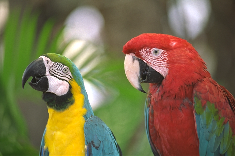
The fit uses center crops of danjacobellis/LSDIR_8k training images; the test image is from danjacobellis/kodak, which is test-only — the fit never sees it. RGB planes are centered to \([-128, 127]\), so \(N = 128\) covers them.
import numpy as np
from datasets import load_dataset

def center_crop(img, side):
    w, h = img.size
    left, top = (w - side) // 2, (h - side) // 2
    return img.crop((left, top, left + side, top + side))

lsdir = load_dataset('danjacobellis/LSDIR_8k', split='train')
fit_set = []
for sample in lsdir:
    img = sample['image'].convert('RGB')
    if min(img.size) < FIT_CROP:
        continue
    arr = np.asarray(center_crop(img, FIT_CROP), np.int64) - 128
    fit_set.append(arr.transpose(2, 0, 1))         # (3, H, W) in [-128, 127]
    if len(fit_set) == FIT_IMAGES:
        break

kodak = load_dataset('danjacobellis/kodak', split='validation')
test_img = kodak[KODAK_INDEX]['image'].convert('RGB')
test_tensor = np.asarray(test_img, np.int64).transpose(2, 0, 1) - 128
import matplotlib.pyplot as plt

display(test_img)
Running the fit#
GGDLPC.fit takes a loader factory: each call returns a fresh iterable of (B, C, *S) integer tensors, and each fitting pass makes one full sweep. At this alphabet size the residual statistics come from a dense joint histogram \(h(S, r)\); the passes log as they run.
import torch
import GGDLPC

def loader_factory():
    batches = [np.stack(fit_set[i:i + 4]) for i in range(0, len(fit_set), 4)]
    return (torch.from_numpy(b) for b in batches)

channels, provenance = GGDLPC.fit(loader_factory, N=N, rank=RANK)
blob = GGDLPC.new_blob(N, RANK, channels, provenance)
GGDLPC fit N=128 rank=2: predictor moments over 4 batches (0s)
GGDLPC fit N=128 rank=2: dense h(S, r) over 4 batches (0s)
GGDLPC fit N=128 rank=2: ch 0: mu=+0.003 a=0.8852 b=0.4220 u=0.692 v=+0.080 wq=[179, 200, -105, -7, -14] bq=-35
GGDLPC fit N=128 rank=2: ch 1: mu=-0.079 a=0.8896 b=0.4631 u=0.818 v=+0.047 wq=[173, 196, -97, -7, -14] bq=-55
GGDLPC fit N=128 rank=2: ch 2: mu=-0.017 a=0.8912 b=0.3859 u=0.628 v=+0.093 wq=[175, 199, -95, -9, -17] bq=-70
for ch in blob['channels']:
    print({k: ch[k] for k in ('channel', 'mu', 'a', 'b', 'u', 'v', 'wq', 'bq')})
{'channel': 0, 'mu': 0.0028657913208007812, 'a': 0.8852414602655242, 'b': 0.42198375831029544, 'u': 0.6924222371621105, 'v': 0.08010766264063081, 'wq': [179, 200, -105, -7, -14], 'bq': -35}
{'channel': 1, 'mu': -0.07900810241699219, 'a': 0.889632505306058, 'b': 0.4630586709942959, 'u': 0.8179560364865117, 'v': 0.04747343083974706, 'wq': [173, 196, -97, -7, -14], 'bq': -55}
{'channel': 2, 'mu': -0.016869544982910156, 'a': 0.8912263157407407, 'b': 0.38588090036727074, 'u': 0.6278194595556764, 'v': 0.09313668363348518, 'wq': [175, 199, -95, -9, -17], 'bq': -70}
Predictor-fitting options#
The predictor pass above is one unconstrained ridge least-squares solve per channel, with an intercept, weights rounded to 1/256 (predictor='ls', the default; every other default reproduces this recipe value for value, which the self-test asserts against golden_fits.json). Since 0.0.3, keyword-only options on GGDLPC.fit select other recipes. The coder cannot tell how the integer weights were chosen: a blob fitted under any option is an ordinary blob, and nothing in the stream, the tables, the engine, or the rate proxy changes.
option |
recipe |
use when |
|---|---|---|
|
ridge LSQ with intercept |
latents and zero-mean sources |
|
the same without the intercept (\(b_q = 0\)) |
the bias is not wanted as a free parameter |
|
weights constrained to sum to exactly one after rounding, no intercept; solved on differenced regressors (\(z - n_0\) on \(n_k - n_0\)) |
records carry large, sign-varying DC offsets (a gravity axis of an accelerometer): the unconstrained solution leaks toward the pooled mean and each record’s residual inherits a bias proportional to its offset |
|
iteratively reweighted least squares toward the absolute-error minimizer ( |
r |
|
each batch row’s mean is subtracted before the predictor moments are accumulated (the law passes still run on the real integers) |
the predictor should be fitted on fluctuations; unsuitable when the coder sees the DC and the weight sum is not one |
|
caller-given integer weights; the predictor pass is skipped |
a predictor chosen elsewhere; only the laws are fitted |
provenance['fit_options'] records the resolved options of every fit and provenance['predictor_weight_sum'] the per-channel sum of \(w_q / 256\). The evidence for when each option wins is experiments/L_fit_options/summary.md; on the image latents fitted here the offsets are small and the sum-to-one constraint changes little.
channels_dc, provenance_dc = GGDLPC.fit(loader_factory, N=N, rank=RANK, log=None,
                                        predictor='ls_dc_invariant')
print('default   ', provenance['fit_options'], provenance['predictor_weight_sum'])
print('dc_invariant', provenance_dc['fit_options'], provenance_dc['predictor_weight_sum'])
for ch, ch_dc in zip(blob['channels'], channels_dc):
    print(f"ch {ch['channel']}: ls wq={ch['wq']} bq={ch['bq']}  |  ls_dc_invariant wq={ch_dc['wq']} bq={ch_dc['bq']}")
default    {'predictor': 'ls', 'bias': True, 'loss': 'l2', 'demean': 'none', 'irls_iters': 0, 'weights_given': False} [0.98828125, 0.98046875, 0.98828125]
dc_invariant {'predictor': 'ls_dc_invariant', 'bias': False, 'loss': 'l2', 'demean': 'none', 'irls_iters': 0, 'weights_given': False} [1.0, 1.0, 1.0]
ch 0: ls wq=[179, 200, -105, -7, -14] bq=-35  |  ls_dc_invariant wq=[180, 200, -105, -6, -13] bq=0
ch 1: ls wq=[173, 196, -97, -7, -14] bq=-55  |  ls_dc_invariant wq=[174, 197, -97, -6, -12] bq=0
ch 2: ls wq=[175, 199, -95, -9, -17] bq=-70  |  ls_dc_invariant wq=[176, 200, -96, -8, -16] bq=0
The causal template and the predictor#
At rank 2 the causal template has five features in canonical order: the two immediate neighbors \(n_0\) (north) and \(n_1\) (west), the diagonal \(p_{01}\), and the distance-2 neighbors \(m_0\), \(m_1\). The predictor is a ridge least-squares regression of each sample on this template plus an intercept, accumulated only where the full template is available, then quantized to fixed-point \(/256\) integers — the arithmetic the C engine runs. The following cell repeats the solve inline:
def shift(x, d, k):
    out = np.zeros_like(x)
    src = [slice(None)] * x.ndim
    dst = [slice(None)] * x.ndim
    src[2 + d] = slice(None, -k)
    dst[2 + d] = slice(k, None)
    out[tuple(dst)] = x[tuple(src)]
    return out

Z = np.stack(fit_set)                     # (T, C, H, W)
feats = [shift(Z, 0, 1), shift(Z, 1, 1),                    # n0, n1
         shift(shift(Z, 0, 1), 1, 1),                       # p01
         shift(Z, 0, 2), shift(Z, 1, 2)]                    # m0, m1

wq_inline, bq_inline = [], []
for c in range(Z.shape[1]):
    cols = [f[:, c, 2:, 2:].ravel().astype(np.float64) for f in feats]
    cols.append(np.ones_like(cols[0]))                      # intercept
    X = np.stack(cols, axis=1)
    y = Z[:, c, 2:, 2:].ravel().astype(np.float64)
    M = X.T @ X
    M += np.eye(M.shape[0]) * (1e-9 * np.trace(M) + 1e-12)  # ridge
    w = np.linalg.solve(M, X.T @ y)
    wq_inline.append(np.round(w[:5] * 256).astype(np.int64))
    bq_inline.append(int(np.round(w[5] * 256)))

for c, ch in enumerate(blob['channels']):
    print(f"channel {c}: fit wq={ch['wq']} bq={ch['bq']}  "
          f"inline wq={wq_inline[c].tolist()} bq={bq_inline[c]}")
    assert np.array_equal(wq_inline[c], ch['wq']) and bq_inline[c] == ch['bq']
channel 0: fit wq=[179, 200, -105, -7, -14] bq=-35  inline wq=[179, 200, -105, -7, -14] bq=-35
channel 1: fit wq=[173, 196, -97, -7, -14] bq=-55  inline wq=[173, 196, -97, -7, -14] bq=-55
channel 2: fit wq=[175, 199, -95, -9, -17] bq=-70  inline wq=[175, 199, -95, -9, -17] bq=-70
Residuals and the pooled statistic#
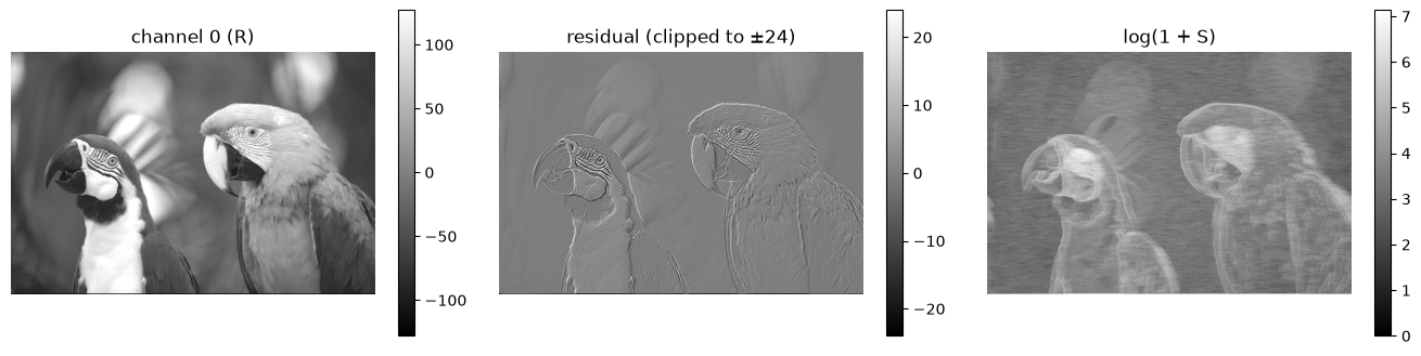
GGDLPC.maps.int_maps is the vectorized torch mirror of the C engine’s integer semantics: fixed-point FIR prediction with an arithmetic-mean fallback where the full template is unavailable, and the pooled statistic \(S = \lfloor 16 (A + w_\text{sum}) / (\text{cnt} + w_\text{cnt}) \rfloor\), where \((A, \text{cnt})\) are the causal template’s absolute differences and \((w_\text{sum}, w_\text{cnt})\) a sliding window over the last 16 coded absolute residuals in scan order. \(S\) estimates the local residual scale in units of \(1/16\) before the sample is coded, from information the decoder also has.
from GGDLPC.maps import int_maps

wq_t = torch.tensor([ch['wq'] for ch in blob['channels']], dtype=torch.int64)
bq_t = torch.tensor([ch['bq'] for ch in blob['channels']], dtype=torch.int64)

pred, res, stat = int_maps(torch.from_numpy(test_tensor)[None], wq_t, bq_t, N, RANK)
pred, res, stat = pred[0].numpy(), res[0].numpy(), stat[0].numpy()

fig, axs = plt.subplots(1, 3, figsize=(13.5, 3.4))
for ax, img, title in zip(axs,
                          (test_tensor[0], res[0].clip(-24, 24), np.log1p(stat[0])),
                          ('channel 0 (R)', 'residual (clipped to ±24)',
                           'log(1 + S)')):
    im = ax.imshow(img, cmap='gray')
    ax.set_title(title)
    ax.set_axis_off()
    plt.colorbar(im, ax=ax)
plt.tight_layout()
The joint histogram \(h(S, r)\)#
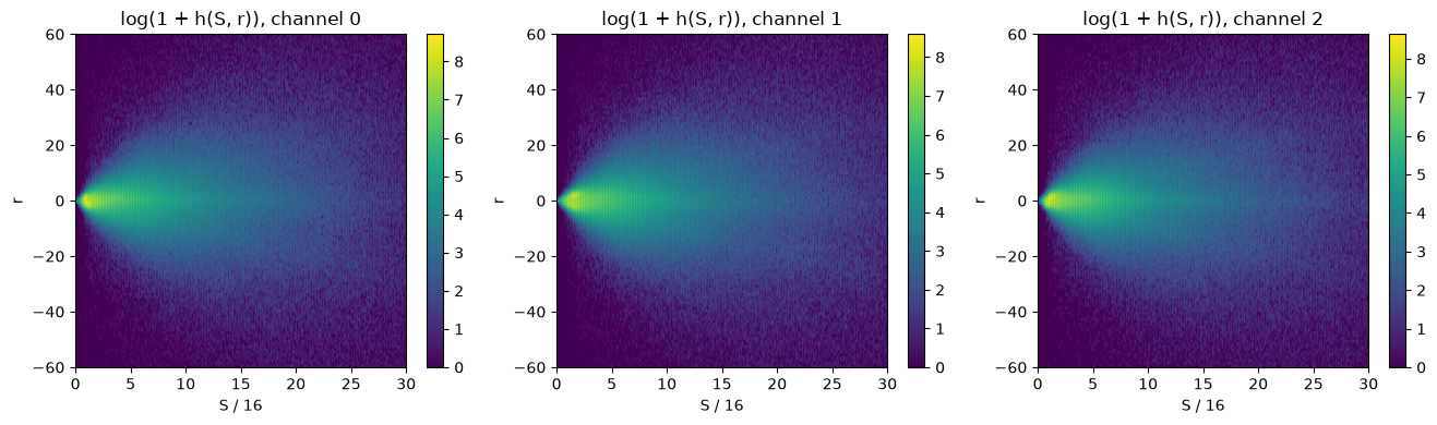
The dense fitting pass reduces the whole fitting set to one 2-D histogram per channel: statistic bin by residual value. Both laws are computed from this histogram.
NSTAT = GGDLPC.stat_cap(N) + 1
NRES = 4 * N + 1                          # residuals span [-2N, 2N]

Zt = torch.from_numpy(Z)
_, res_all, stat_all = int_maps(Zt, wq_t, bq_t, N, RANK)
res_all, stat_all = res_all.numpy(), stat_all.numpy()

hist = np.zeros((Z.shape[1], NSTAT, NRES), np.int64)
for c in range(Z.shape[1]):
    np.add.at(hist[c], (stat_all[:, c].ravel(), res_all[:, c].ravel() + 2 * N), 1)

fig, axs = plt.subplots(1, 3, figsize=(13.5, 4))
for c in range(3):
    im = axs[c].imshow(np.log1p(hist[c][:480, 2 * N - 60:2 * N + 61]).T, aspect='auto',
                       origin='lower', extent=(0, 30, -60, 60))
    axs[c].set_title(f'log(1 + h(S, r)), channel {c}')
    axs[c].set_xlabel('S / 16')
    axs[c].set_ylabel('r')
    plt.colorbar(im, ax=axs[c])
plt.tight_layout()
The scale law#
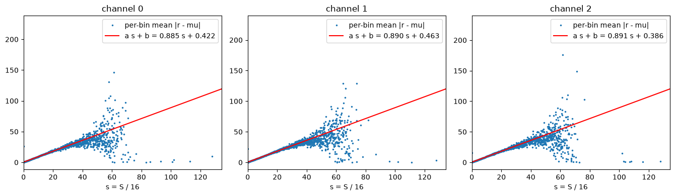
Within each statistic bin, the mean absolute deviation of the residual is nearly affine in \(S/16\): the statistic predicts the residual scale. The law \((a, b)\) is a weighted least-squares line through the per-bin means, weighted by bin occupancy — the same computation fit performs on this histogram.
rvals = np.arange(NRES) - 2 * N
t16 = np.arange(NSTAT) / 16.0

fig, axs = plt.subplots(1, 3, figsize=(13.5, 4))
for c in range(3):
    h = hist[c]
    n_t = h.sum(axis=1).astype(np.float64)
    mu_c = float((h.sum(axis=0) * rvals).sum() / n_t.sum())
    m_t = (h * np.abs(rvals - mu_c)).sum(axis=1) / np.maximum(n_t, 1.0)
    w = n_t
    sw, swx, swy = w.sum(), (w * t16).sum(), (w * m_t).sum()
    swxx, swxy = (w * t16 * t16).sum(), (w * t16 * m_t).sum()
    den = sw * swxx - swx * swx
    a_c = (sw * swxy - swx * swy) / den
    b_c = (swy - a_c * swx) / sw
    a_c, b_c = max(a_c, 0.0), max(b_c, 1 / 16)
    ch = blob['channels'][c]
    print(f"channel {c}: inline mu={mu_c:+.4f} a={a_c:.4f} b={b_c:.4f}   "
          f"fit mu={ch['mu']:+.4f} a={ch['a']:.4f} b={ch['b']:.4f}")
    assert np.allclose([mu_c, a_c, b_c], [ch['mu'], ch['a'], ch['b']])
    occupied = n_t > 0
    axs[c].plot(t16[occupied], m_t[occupied], '.', ms=3, label='per-bin mean |r - mu|')
    axs[c].plot(t16, a_c * t16 + b_c, 'r', label=f'a s + b = {a_c:.3f} s + {b_c:.3f}')
    axs[c].set_title(f'channel {c}')
    axs[c].set_xlabel('s = S / 16')
    axs[c].set_xlim(0, t16[occupied].max() * 1.05)
    axs[c].legend()
plt.tight_layout()
channel 0: inline mu=+0.0029 a=0.8852 b=0.4220   fit mu=+0.0029 a=0.8852 b=0.4220
channel 1: inline mu=-0.0790 a=0.8896 b=0.4631   fit mu=-0.0790 a=0.8896 b=0.4631
channel 2: inline mu=-0.0169 a=0.8912 b=0.3859   fit mu=-0.0169 a=0.8912 b=0.3859
The shape law#
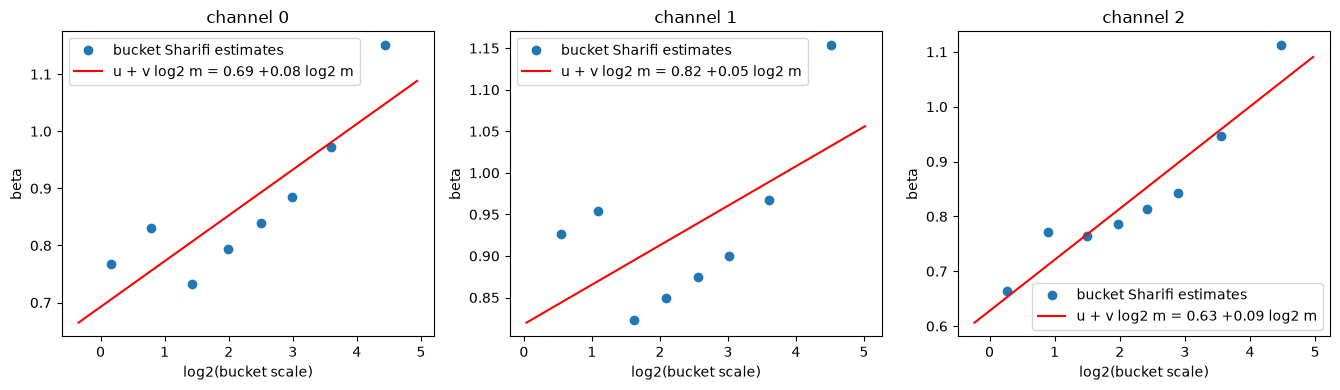
The GGD shape is estimated per occupancy bucket with the Sharifi–Leon-Garcia moment method: \(\rho = E(x-\mu)^2 / (E|x-\mu|)^2\) determines \(\beta\) through a gamma-function identity. The statistic axis is cut into \(K = 8\) equal-occupancy buckets, each populous enough for a stable estimate, and the law \((u, v)\) is a weighted affine fit of the bucket shapes against \(\log_2\) of the bucket scale.
from scipy.optimize import brentq
from scipy.special import gammaln

def sharifi_beta(rho):
    def f(b):
        return (gammaln(1 / b) + gammaln(3 / b) - 2 * gammaln(2 / b)) - np.log(rho)
    if f(0.05) < 0:
        return 0.05
    if f(10.0) > 0:
        return 10.0
    return brentq(f, 0.05, 10.0, xtol=1e-6)

K_BETA, MIN_OCC = 8, 10_000

fig, axs = plt.subplots(1, 3, figsize=(13.5, 4))
for c in range(3):
    h = hist[c].astype(np.float64)
    marg = h.sum(axis=1)
    cum = np.cumsum(marg)
    edges = np.array([int(np.searchsorted(cum, cum[-1] * i / K_BETA))
                      for i in range(1, K_BETA)])
    buckets = np.searchsorted(edges, np.arange(NSTAT), side='right')
    hb = np.zeros((K_BETA, NRES))
    np.add.at(hb, buckets, h)
    xs, ys, ws = [], [], []
    for kb in range(K_BETA):
        row = hb[kb]
        nn = row.sum()
        if nn < MIN_OCC:
            continue
        mu_b = (row * rvals).sum() / nn
        e1 = max((row * np.abs(rvals - mu_b)).sum() / nn, 1e-3)
        e2 = (row * (rvals - mu_b) ** 2).sum() / nn
        xs.append(np.log2(e1))
        ys.append(sharifi_beta(max(e2 / max(e1 * e1, 1e-12), 1.0001)))
        ws.append(nn)
    x, y, w = map(np.asarray, (xs, ys, ws))
    A = np.stack([np.ones_like(x), x], axis=1) * np.sqrt(w)[:, None]
    u_c, v_c = np.linalg.lstsq(A, y * np.sqrt(w), rcond=None)[0]
    ch = blob['channels'][c]
    print(f"channel {c}: inline u={u_c:.4f} v={v_c:+.4f}   "
          f"fit u={ch['u']:.4f} v={ch['v']:+.4f}")
    assert np.allclose([u_c, v_c], [ch['u'], ch['v']])
    axs[c].plot(x, y, 'o', label='bucket Sharifi estimates')
    xx = np.linspace(x.min() - 0.5, x.max() + 0.5, 50)
    axs[c].plot(xx, u_c + v_c * xx, 'r', label=f'u + v log2 m = {u_c:.2f} {v_c:+.2f} log2 m')
    axs[c].set_title(f'channel {c}')
    axs[c].set_xlabel('log2(bucket scale)')
    axs[c].set_ylabel('beta')
    axs[c].legend()
plt.tight_layout()
channel 0: inline u=0.6924 v=+0.0801   fit u=0.6924 v=+0.0801
channel 1: inline u=0.8180 v=+0.0475   fit u=0.8180 v=+0.0475
channel 2: inline u=0.6278 v=+0.0931   fit u=0.6278 v=+0.0931
The fitted laws against the empirical conditionals#
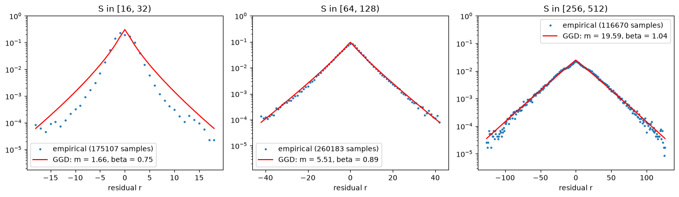
The scalars replace the histogram: at a statistic value \(s\), the scale law gives \(\hat m = a s + b\), the shape law gives \(\beta\), and the analytic GGD with those parameters is the conditional the coder uses (the next chapter generates the tables from it). Three statistic bands of channel 0, empirical residual conditional against the law-generated GGD:
from scipy.special import gammainc

def ggd_cdf(x, beta):
    return 0.5 + 0.5 * np.sign(x) * gammainc(1.0 / beta, np.abs(x) ** beta + 1e-300)

ch = blob['channels'][0]
bands = ((16, 32), (64, 128), (256, 512))
fig, axs = plt.subplots(1, 3, figsize=(13.5, 4))
for ax, (s_lo, s_hi) in zip(axs, bands):
    rows = hist[0][s_lo:s_hi].astype(np.float64)
    occ = rows.sum(axis=1)
    emp = rows.sum(axis=0)
    n = emp.sum()
    emp = emp / n
    s_mid = (occ * (np.arange(s_lo, s_hi) / 16.0)).sum() / occ.sum()
    m = max(ch['a'] * s_mid + ch['b'], 1 / 16)
    beta = float(np.clip(ch['u'] + ch['v'] * np.log2(m), 0.2, 4.0))
    alpha = np.exp(gammaln(1 / beta) - gammaln(2 / beta)) * m
    model = np.maximum(ggd_cdf((rvals + 0.5 - ch['mu']) / alpha, beta)
                       - ggd_cdf((rvals - 0.5 - ch['mu']) / alpha, beta), 0.0)
    r_lim = int(min(2 * N, np.ceil(6 * m) + 8))
    sel = np.abs(rvals) <= r_lim
    ax.semilogy(rvals[sel], np.where(emp[sel] > 0, emp[sel], np.nan), '.', ms=4,
                label=f'empirical ({int(n)} samples)')
    ax.semilogy(rvals[sel], model[sel], 'r',
                label=f'GGD: m = {m:.2f}, beta = {beta:.2f}')
    ax.set_ylim(max(0.3 / n, 1e-8), 1)
    ax.set_title(f'S in [{s_lo}, {s_hi})')
    ax.set_xlabel('residual r')
    ax.legend()
plt.tight_layout()
The blob#
The blob is the entire persistent model: the scalars and predictor integers per channel plus provenance, as one JSON-able dict. GGDLPC.Codec(blob) generates every table from it at construction; the next chapter performs that generation inline.
import json

print(json.dumps({k: blob[k] for k in ('version', 'N', 'rank', 'channels')}, indent=1)[:1500])
{
 "version": 1,
 "N": 128,
 "rank": 2,
 "channels": [
  {
   "channel": 0,
   "mu": 0.0028657913208007812,
   "a": 0.8852414602655242,
   "b": 0.42198375831029544,
   "u": 0.6924222371621105,
   "v": 0.08010766264063081,
   "wq": [
    179,
    200,
    -105,
    -7,
    -14
   ],
   "bq": -35,
   "n_samples": 1048576
  },
  {
   "channel": 1,
   "mu": -0.07900810241699219,
   "a": 0.889632505306058,
   "b": 0.4630586709942959,
   "u": 0.8179560364865117,
   "v": 0.04747343083974706,
   "wq": [
    173,
    196,
    -97,
    -7,
    -14
   ],
   "bq": -55,
   "n_samples": 1048576
  },
  {
   "channel": 2,
   "mu": -0.016869544982910156,
   "a": 0.8912263157407407,
   "b": 0.38588090036727074,
   "u": 0.6278194595556764,
   "v": 0.09313668363348518,
   "wq": [
    175,
    199,
    -95,
    -9,
    -17
   ],
   "bq": -70,
   "n_samples": 1048576
  }
 ]
}