Sensor-Embedded Autoencoding with One-Time Transcode#
Robotic platforms routinely capture vast amounts of visual data at high resolution using low-cost, low-power image sensors. Yet, limited bandwidth and on-device compute resources prevent full utilization when transmitted via conventional codecs like JPEG/MPEG. Newer codecs, like AV1/AVIF, improve the rate-distortion trade-off, but demand far more resources for encoding, impractical without custom ASICs. Recent asymmetric autoencoders deliver high quality under extreme power and bandwidth constraints, but add prohibitive decoding cost and use bespoke formats that ignore decades of infrastructure built around standards like JPEG. To address these limitations, we introduce SEAOTTER, a compression framework for cloud robotics based on a sensor-embedded autoencoder paired with a one-time transcode for efficient reconstruction. Because the sensor, cloud, and consumer stages face very different power and bandwidth budgets, SEAOTTER combines the compactness of a learned latent with the broad usability of a standard JPEG file. Since naive transcoding degrades performance, we propose a learnable JPEG color and quantization transform that enables increased accuracy for global, dense, and vision-language-based perception. Using SEAOTTER, we train both general-purpose and task-aware transcoding pipelines for a pre-trained, frozen encoder. At a compression ratio of 200:1 and compared to AVIF, we observe \(7\times\) faster encoding, \(3.5\times\) faster decoding, and +8% ImageNet top-1 accuracy, while retaining compatibility with JPEG infrastructure. Our code is available at UT-SysML/seaotter.
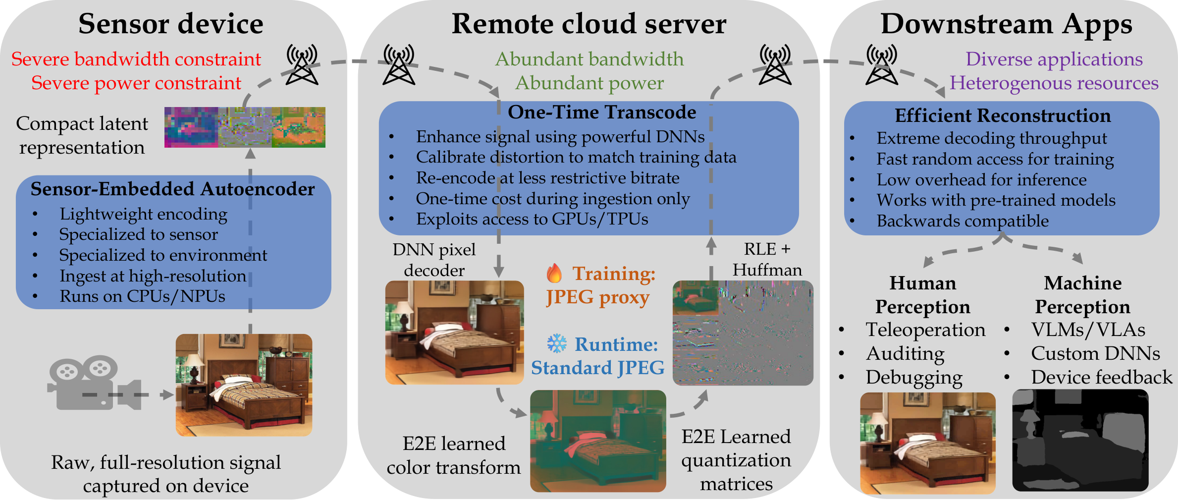
Fig. 24 Overview of SEAOTTER design and workflow.#
Introduction#
The staggering economic scale of the smartphone market has driven extraordinary advances in image sensing: modern low-cost, low-power sensors let small, battery-powered robots and wearables capture billions of pixels per second at a fidelity once reserved for earth-observation satellites, consuming on the order of \(10^{-11}\) joules per pixel (Chen et al., 2014, Kim et al., 2022). Yet fully utilizing these information-dense signals on-device is prohibitive, because the most capable ViT- and CNN-based perception systems require FLOPs that scale super-linearly with resolution (Beyer, 2024); it is common to instead use only low-resolution feeds and discard the rest. Cloud-robotics approaches—remote inference (Jacobellis et al., 2026), split inference (Kang et al., 2017, Matsubara et al., 2022), and collaborative inference (Gao et al., 2025, Wang et al., 2024)—offload this computation to datacenters where power is abundant, but on-device power and bandwidth then demand extreme compression to reach the cloud. For example, a 1080p 30 fps stream over a 25 Mbps Wi-Fi channel requires a compression ratio of about 60:1, and a 480p stream over a 1 Mbps BLE channel about 288:1 (Balasubramanian et al., 2009, Carroll and Heiser, 2010, Gupta et al., 2024, Tosi et al., 2017). Conventional codecs like JPEG/MPEG meet these ratios only at severe perceptual cost (Jacobellis et al., 2024); newer standards (AV1/AVIF) and decoding-efficient asymmetric autoencoders (DE-AAEs) (Yang and others, 2023) improve the rate–distortion trade-off but demand prohibitively expensive encoding. Encoding-efficient asymmetric autoencoders (EE-AAEs) (Hojjat et al., 2025, Jacobellis and Yadwadkar, 2025, Jacobellis and Yadwadkar, 2026) invert this trade-off, pairing a lightweight encoder with an expensive DNN decoder that removes the artifacts of severe dimension reduction. We build on FRAPPE (Jacobellis and Yadwadkar, 2026), whose encoder costs only 10–100 MAC/pixel—at low bitrates, less than JPEG.
These EE-AAEs, however, are impractical on the consumer side: their DNN decoders are costly to run, and their bespoke latents are incompatible with the decades of infrastructure built around JPEG—ML frameworks, fast dataloaders, web browsers, and hardware codecs baked into ASICs and SoCs. Decoding cost is especially punishing under the encode-once, decode-many lifecycle of modern workloads: a training run re-reads each file once per epoch with fresh augmentations, so any per-decode overhead is multiplied by the consumption count. A single up-front transcode into a cheaper-to-decode artifact is therefore favorable whenever a file is read more than once—which is why JPEG/M-JPEG remains ubiquitous across robotics.
To address these limitations, we introduce SEAOTTER (Fig. 24), a sensor-embedded autoencoder with a one-time transcode for efficient reconstruction that reconciles resource-constrained sensors with data-hungry consumers through three goals detailed in Negative-Distortion Transcoding via Jointly Trained JPEG Proxy: high-throughput sensor-side encoding, end-to-end task adaptability, and universal consumer-side compatibility.
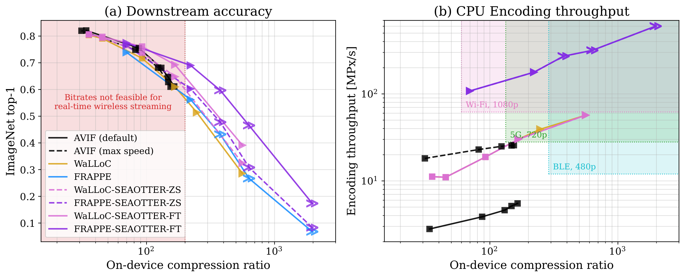
Fig. 25 (a) Classification accuracy and (b) CPU encoding throughput vs. on-device compression ratio. Shaded regions mark the compression ratio and throughput needed for 1080p/30 over Wi-Fi (25 Mbps), 720p/30 over 5G (5 Mbps), and 480p/30 over BLE (1 Mbps). \(\blacksquare\), \(>\), and \(\gg\) mark poor, fair, and excellent on-device suitability; configurations in the red region are poorly suited.#
Sensor-embedded encoding under extreme resource constraints. Robotic, wearable, and remote-sensing platforms run their image sensors against strict power, thermal, and uplink-bandwidth budgets, so the sensor-side encoder must spend orders of magnitude less compute per pixel than a hyperprior (Ballé et al., 2018, Minnen et al., 2018), a vanilla JPEG encoder, or modern codecs like AVIF, whose run-time rate-distortion optimization and multi-stage in-loop filtering reach a per-pixel cost that production deployments meet only with dedicated hardware encoders (Bossen et al., 2021). SEAOTTER instead uses an EE-AAE (Hojjat et al., 2025, Jacobellis and Yadwadkar, 2025, Jacobellis and Yadwadkar, 2026) built on a pre-trained FRAPPE codec (Jacobellis and Yadwadkar, 2026), chosen for its high encoding efficiency and low-overhead variable-rate and progressive coding—crucial for systems operating under fluctuating bandwidth and shared CPU/NPU load.
Learning specialized representations via end-to-end optimization. To support diverse robotics applications, the codec must handle arbitrary sensors and conditions—high motion, aerial views, poor lighting, fish-eye distortion. JPEG uses fixed color transforms and quantization matrices tuned to human perception; SEAOTTER instead learns these from data while staying compatible with standard JPEG hardware and software, specializing to the camera, environment, and downstream model. We freeze the FRAPPE encoder and fine-tune the FRAPPE decoder and JPEG color/quantization parameters; jointly optimizing the encoder could yield further gains.
Flexible and efficient decoding. The cloud-side transcode produces standard-compliant JPEG files with the custom quantization matrices embedded in metadata. The standard RGB-YUV color transform is forgone, and the codec is sandwiched between a learned color transform and a companding nonlinearity that enforces the limited dynamic range. For bespoke machine-vision applications, decoding is then faster than standard JPEG, since the inverse color transform can be skipped to operate directly in the learned color space (Ehrlich and Davis, 2019, Gueguen et al., 2018). For pre-trained models that accept sRGB inputs and cannot be fine-tuned (e.g., billion-parameter foundation models, VLMs, and VLAs), the only overhead is a single post-filter (\({\sim}81\) MACs/pixel).
Contributions. Using SEAOTTER, we (i) frame cloud-robotics compression as a three-way sensor / cloud / consumer asymmetry under an encode-once, decode-many lifecycle; (ii) introduce an end-to-end learned JPEG codec—color transform, quantization, and rate proxy trained de novo—that beats the ITU T.81 tables; and (iii) show across global, dense, and vision-language tasks that the one-time transcode increases downstream accuracy over the underlying autoencoder while emitting standard JPEG files (Fig. 25).
Negative-Distortion Transcoding via Jointly Trained JPEG Proxy#
Overview and workflow. SEAOTTER’s pipeline has three stages separated by two compressed bitstreams: a frozen sensor-embedded analysis transform produces a quantized \(\text{int}8\) latent that is losslessly compressed and transmitted over the wireless uplink; at the cloud, a heavy synthesis transform reconstructs an intermediate pixel image, which an end-to-end learned JPEG codec re-encodes as a standard JPEG file—a transcode paid exactly once per captured frame. The on-disk artifact is thereafter a plain JPEG file, decoded by every downstream consumer with a vanilla JPEG decode followed by a single learned inverse color transform. Fig. 24 overviews the workflow, described next.
Let \(x\in\mathbb{R}^{3\times H\times W}\) denote an input RGB image, normalized to \([-1,1]\). SEAOTTER composes a sensor-side analysis transform \(\mathcal{G}_{\!A}\), a lossless transmission channel \(\mathcal{C}\), a cloud-side synthesis transform \(\mathcal{G}_{\!S}\), a learned color transform \(\mathcal{F}\) with inverse \(\mathcal{F}^{-1}\), and a JPEG codec \(\mathcal{J}_Q\) parameterized by a learned quantization matrix \(Q\):
Here \(\mathcal{G}_{\!A}\) is the frozen FRAPPE encoder and \(\mathcal{G}_{\!S}\) the matching FRAPPE decoder (fine-tuned below); the lossless channel \(\mathcal{C}\) packages JPEG-LS (Weinberger et al., 2000) entropy coding, uplink transmission, and cloud-side decoding, so for Eq. (10) it is the identity; \((\mathcal{F}, \mathcal{F}^{-1})\) is the invertible learned color transform; and \(\mathcal{J}_Q\) is the single inherently lossy step, a standard JPEG encode–decode round-trip with the learned quantization matrix \(Q\).
FRAPPE encoder for variable rate compression under extreme resource constraints. \(\mathcal{G}_{\!A}\) is a FRAPPE (Jacobellis and Yadwadkar, 2026) encoder, which projects input patches of varying scales (from \(32{\times}32\) to \(4{\times}4\)) to scalar values. Its cost is dominated by the linear projections and amounts to roughly \(10\)–\(100\) MAC/pixel depending on the operating point—two orders of magnitude lower than the smallest learned hyperprior codecs (Ballé et al., 2018, Minnen et al., 2018). FRAPPE’s residual training procedure sorts the latent channels in coarse-to-fine order, so a single set of encoder weights serves every supported rate point (\(n\in\{3,6,9,12,15\}\)): the sensor selects its operating point by transmitting a prefix of the channels rather than re-encoding. We freeze \(\mathcal{G}_{\!A}\) throughout, matching the asymmetric-capacity stance of WaLLoC (Jacobellis and Yadwadkar, 2025) and LiVeAction (Jacobellis and Yadwadkar, 2026), where sensor-side compute is a hard budget rather than a tunable axis. After encoding, the int8 latents are losslessly compressed (the framework is agnostic to the specific lossless codec).
Fine-tuned FRAPPE decoder for application-specific signal enhancement and calibration. The cloud-side synthesis transform \(\mathcal{G}_{\!S}\) is the FRAPPE decoder (\({\sim}57\text{M}\) parameters). Unlike \(\mathcal{G}_{\!A}\), \(\mathcal{G}_{\!S}\) is fine-tuned against the downstream task loss with the encoder still frozen; its RGB output drifts toward a distribution that a JPEG-pretrained consumer-side backbone (Accuracy Gains from Negative-Distortion Transcoding) reads more accurately. Because \(\mathcal{G}_{\!A}\) is frozen, every fine-tuned \(\mathcal{G}_{\!S}\) snapshot is interchangeable at runtime: the same transmitted latent decodes to different RGB outputs depending on the chosen snapshot, so a single uplink stream can serve multiple downstream tasks simultaneously. The fine-tune deliberately sacrifices pixel-domain reconstruction PSNR for higher downstream accuracy after the transcode, specializing \(\mathcal{G}_{\!S}\)’s output for the JPEG step that follows.
JPEG sandwich. The cloud-side decoder’s RGB output enters a learned JPEG sandwich: a forward color transform \(\mathcal{F}\) into a JPEG-friendly representation, a standard JPEG encode with a learned \(3{\times}8{\times}8\) quantization matrix \(Q\), and an inverse color transform \(\mathcal{F}^{-1}\) at the consumer. The closest prior art is the sandwiched codec of Guleryuz et al. (2021), Guleryuz et al. (2024), which wraps U-Net pre- and post-processors around a standard codec, trained end-to-end on a per-image rate–distortion proxy. SEAOTTER differs in three ways: (i) its color transform \(\mathcal{F}\) is a lightweight \(3{\times}3\) convolution plus companding rather than a U-Net, so the consumer-side decode pays at most a vanilla JPEG-decode cost plus a few thousand floating-point operations per pixel; (ii) it is trained de novo with no codec warm-starts, so its win over standard JPEG comes from representation rather than bookkeeping; and (iii) a single learned \((\mathcal{F}, \mathcal{F}^{-1})\) pair is shared across all \(K\) rate points, with \(K\) independent quantization matrices \(Q^{(1)},\dots,Q^{(K)}\) specializing the per-rate behavior. Fig. 26 shows the resulting workflow.
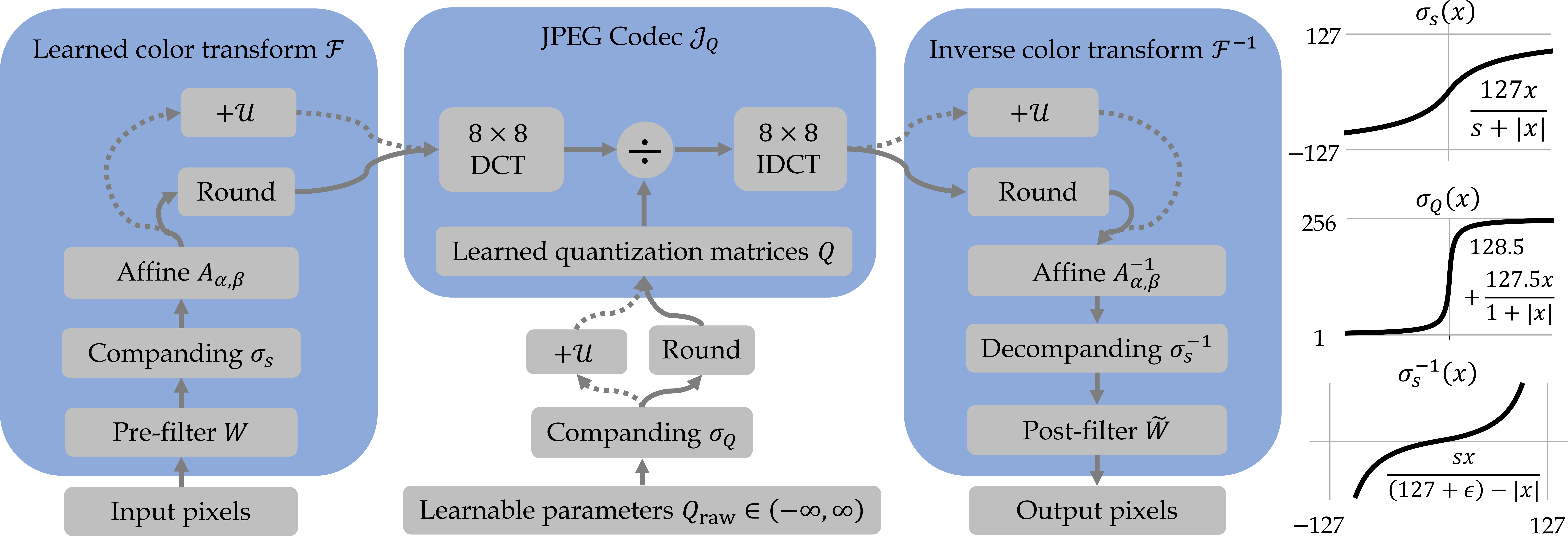
Fig. 26 JPEG workflow with learned color transform and quantization and visualization of companding/decompanding functions. Dotted lines indicate the signal path during training.#
De novo learnable wrapper filter and color transform. \(\mathcal{F}\) composes three operators: a \(3{\times}3\) wrapper filter \(\mathrm{Conv}_W\) with learnable kernel \(W\)—a full \(3\)-input, \(3\)-output convolution that jointly filters spatially and mixes the three RGB channels, so it is this operator (not the per-channel stages that follow) that realizes the learned color space—a per-channel softsign companding \(\sigma_s\) with learnable scale \(s\in\mathbb{R}^3_+\) that confines each channel to the signed 8-bit range \((-127, 127)\), and a per-channel affine \(A_{\alpha,\beta}\) with learnable scale \(\alpha\in\mathbb{R}^3\) and offset \(\beta\in\mathbb{R}^3\) that packs the result into the unsigned 8-bit range \([0, 255]\):
where \(\mathcal{F}^{-1}\) mirrors \(\mathcal{F}\) but with an independently-learned wrapper-filter kernel \(\widetilde W\) (a \(3{\times}3\) convolution is not in general algebraically invertible). \(A_{\alpha, \beta}^{-1}\) and \(\sigma_s^{-1}\) are the closed-form algebraic inverses of the corresponding forward operators, with \(\alpha, \beta, s\) shared between \(\mathcal{F}\) and \(\mathcal{F}^{-1}\). The unit-step rounding at the JPEG codec’s boundaries is handled by the canonical three-mode contract of the hyperprior codecs (Ballé et al., 2017, Ballé et al., 2018, Minnen et al., 2018): during training it is replaced with independent additive uniform noise \(u\sim\mathcal{U}[-\tfrac{1}{2},\tfrac{1}{2}]\), during evaluation it uses the continuous output of the preceding operator, and at deployment an explicit \(\mathrm{round}(\cdot)\) is applied outside the forward pass. The softsign companding inside \(\mathcal{F}\) confines its pre-quantization output to the 8-bit range regardless of input magnitude, so the contract holds for arbitrary pixel-domain dynamic ranges without per-sensor calibration.
All learnable parameters of \(\mathcal{F}\) and \(\mathcal{F}^{-1}\)—the wrapper-filter kernels \(W\) and \(\widetilde W\), the softsign scales \(s\), and the affine \((\alpha, \beta)\)—are initialized so that the composed map is approximately the algebraic identity at step zero, not the JFIF \(\text{RGB}{\to}\text{YCbCr}\) matrix: warm-starting from JFIF would have the network deviate from the codec we are trying to displace rather than discover a color transform, so with identity initialization the only inductive bias is the architectural shape and everything chromatic falls out of the rate–distortion loss on data. At inference time, \(\mathcal{F}\)’s three-channel output is written byte-for-byte into the JPEG file with subsampling=0 (true \(4{:}4{:}4\)); since the channels are not chroma in the conventional sense, the JPEG decoder must skip the standard \(\text{YCbCr}{\to}\text{RGB}\) color conversion. Both options—subsampling=0 and the skipped color conversion—are standard settings exposed by any compliant JPEG implementation, so the on-disk artifact remains decodable by any standards-compliant codec. We verified that, with identity weights, this gives a bit-exact \(\text{RGB}{\leftrightarrow}\text{RGB}\) round-trip.
De novo learnable DCT-domain quantization matrices. For each rate point \(k=1,\dots,K\), an unconstrained \(3{\times}8{\times}8\) parameter tensor \(Q^{(k)}_{\text{raw}}\) maps to a JPEG quantization matrix in the open range \((1,256)\) via a softsign-plus-affine reparameterization,
During training, \(Q^{(k)}\) is the continuous divisor of the \(8{\times}8\) block DCT; at deployment it is rounded and clamped to integers in \([1,255]\). The softsign-plus-affine parameterization is borrowed from FRAPPE’s encoder companding: it keeps the gradient finite as \(Q^{(k)}\) approaches either boundary of the JPEG-legal range. Per-rate independence lets each \(Q^{(k)}\) specialize to its operating point, while the shared \((\mathcal{F}, \mathcal{F}^{-1})\) keeps sensor- and consumer-side costs constant across rates. The learned \(Q^{(k)}\) matrices and the resulting (approximately YCgCo) color space are visualized in Fig. 27.
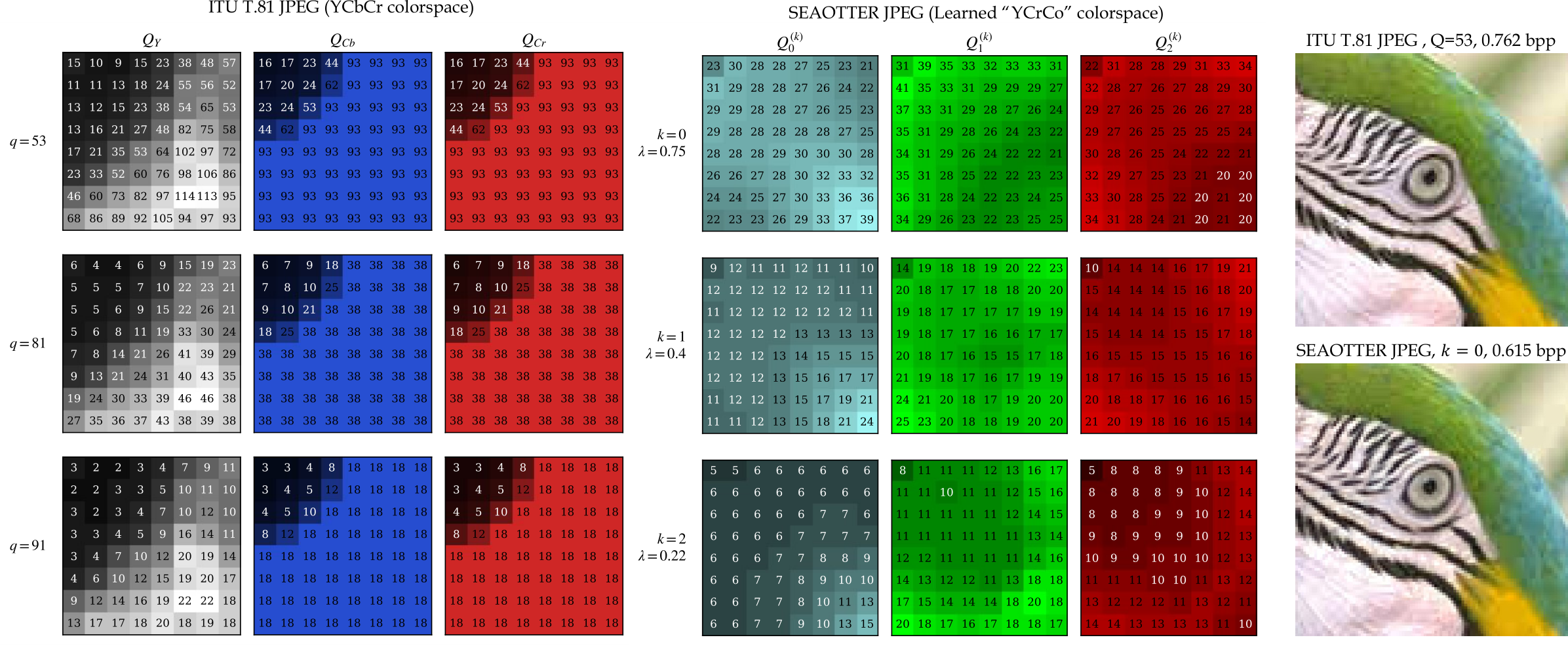
Fig. 27 Learned per-rate DCT-domain quantization matrices \(Q^{(k)}\) for \(k=0,1,2\) (top row) alongside the matched-bpp ITU T.81 4:4:4 quantization tables (bottom row). Per-channel colormap hues are derived from \(\mathcal{F}\)’s learned RGB-mixing kernel; the resulting color space coincides with YCgCo up to per-channel sign.#
Improved JPEG rate proxy. End-to-end training requires a differentiable proxy for the JPEG file size the codec actually produces. We use a sparsity-aware run-length surrogate that models JPEG’s zigzag AC coding: per \(8{\times}8\) block, the bit count is a smooth nonzero gate \(\tanh(c_k^2)\) times \(\log_2\!\bigl(1+|c_k|/Q^{(k)}_k\bigr)\) plus a fixed Huffman-overhead constant, summed over all blocks. This is closely related to the \(\log\!\bigl(1+|x_i|/\Delta\bigr)\) proxy of Guleryuz et al. (2021), with two changes: the soft gate \(\tanh(c_k^2)\) captures the dominant cost of an AC block—whether its coefficients fall within the zero run—and the per-block overhead constant absorbs the Huffman-table bits the bitstream-level proxies omit. A single per-rate scalar \(\alpha^{(k)}\), fit on held-out images, calibrates the surrogate to the real JPEG bits-per-pixel of a standards-compliant encoder; we denote the calibrated proxy \(\mathrm{bpp}^{(k)}(x, Q^{(k)})\).
De novo training of JPEG color and quantization. We train the shared color-transform pair \((\mathcal{F}, \mathcal{F}^{-1})\) and the \(K\) rate-specific quantization matrices \(Q^{(1)},\dots,Q^{(K)}\) jointly, end-to-end, against a multi-rate rate–distortion objective:
where \(\hat{x}_k\) is the reconstruction at rate point \(k\) under the shared \((\mathcal{F}, \mathcal{F}^{-1})\) pair and the rate-specific \(Q^{(k)}\), \(\mathrm{bpp}^{(k)}\) is the calibrated rate proxy, \(\lambda_k>0\) is the Lagrange multiplier trading rate against distortion, and \(w_k>0\) is a per-rate loss weight that arbitrates between rate paths when one would otherwise dominate the gradient. The shared pair is updated by gradients from all \(K\) terms of Eq. (13) simultaneously, so the color transform learns a rate-agnostic representation; each \(Q^{(k)}\) receives gradient only from its own term, so the quantization matrices specialize to their operating points.
The codec is trained de novo: \((\mathcal{F}, \mathcal{F}^{-1})\) is initialized to the algebraic identity (no JFIF warm-start), each \(Q^{(k)}\) is initialized from random Gaussian noise (no quality=Q warm-start), and the JPEG standard’s precomputed Huffman tables are used at runtime instead of per-image optimized tables. Full training details, including the headline \(K{=}3\) rate weights \((\lambda_k, w_k)\), are given in Training recipe.
Optional inverse color transform and post-filter. The consumer-side decode is a vanilla JPEG decode followed by \(\mathcal{F}^{-1}\), which recovers the displayable RGB from the three-channel \(\text{uint}8\) output. Crucially, \(\mathcal{F}^{-1}\) is optional: downstream applications that train or fine-tune their own consumer-side model can skip it and operate directly on the JPEG-decoded coefficients, analogous to prior work on JPEG-domain learning systems that consume YUV (or YCoCg) directly (Ehrlich and Davis, 2019, Gueguen et al., 2018)—the skipped inverse-conv is absorbed into the first layer of the downstream model with no loss of expressivity. SEAOTTER therefore coexists with both legacy JPEG-consuming pipelines (which apply \(\mathcal{F}^{-1}\)) and JPEG-domain learning pipelines (which skip it).
Accuracy Gains from Negative-Distortion Transcoding#
We evaluate SEAOTTER in terms of the rate–distortion–complexity trade-off. Rate is measured in bits per pixel (bpp), reported as both the transmission rate (tbpp, uploaded from the sensor) and the storage rate (sbpp, the transcoded JPEG file); the compression ratio is \(\mathrm{CR} = 24/\mathrm{bpp}\). Distortion is measured via standard metrics (PSNR, SSIM (Wang et al., 2004), LPIPS (Zhang et al., 2018), DISTS (Ding et al., 2020)) and downstream task accuracy, and complexity via on-device CPU encoding throughput (megapixels per second). We compare against AVIF, WaLLoC, and FRAPPE, and evaluate both a zero-shot SEAOTTER pipeline (pre-trained for MSE on a general-purpose dataset (Li et al., 2023)) and a task-specific fine-tuned pipeline. We additionally evaluate the learned JPEG codec as a standalone system against the standard ITU T.81 (ITU-T, 1992) colorspace and quantization tables, with and without chroma subsampling.
Models, datasets, and task-specific performance metrics.
We evaluate downstream task accuracy on three tasks chosen to span global, dense, and VLM-style inference. For global classification (cls), we use ImageNet val (\(50{,}000\) images) (Deng et al., 2009) with a ConvNeXt-Tiny teacher (Liu et al., 2022), reporting top-1/top-5 accuracy. For dense prediction (seg), we use ADE20K val (\(2{,}000\) images) (Zhou et al., 2017) with a UperNet-ConvNeXt-Tiny teacher (Xiao et al., 2018), reporting mIoU. For VLM/VLA-style zero-shot prediction (clip), we use ImageNet val with the SigLIP-2 base-patch16-naflex encoder (Tschannen et al., 2025), reporting zero-shot top-1. Preprocessing is squash to the task resolution (cls \(384^2\), seg \(512^2\)) or naflex (clip), which also sets the bpp denominator. Codec baselines are AVIF (default and max-speed, s10), FRAPPE, and WaLLoC; SEAOTTER variants are denoted SEAOTTER-ZS (zero-shot sandwich) and SEAOTTER-FT (decoder + sandwich fine-tuned for the target task). Standalone-codec baselines use ITU T.81 with and without chroma subsampling (Standalone learned JPEG vs ITU T.81 on Kodak). Teacher checkpoint IDs, naflex hyperparameters, the per-task no-codec accuracy ceilings, and timing hardware are reported in Experiment details.
Figure 25 summarizes the rate–accuracy–throughput trade-off of SEAOTTER variants against AVIF, WaLLoC, and FRAPPE; Figure 29 adds reconstruction-quality axes and Figure 30 the storage-rate axis; Figure 28 gives a multi-axis overview. Table 16 groups three task subsections (cls, seg, clip) and within each reports every pipeline at a single per-task matched-rate operating point: FRAPPE / SEAOTTER variants stay at \(n{=}12\), and each conventional baseline (AVIF, AVIF max-speed, WaLLoC) uses the lowest-bpp op still strictly above FRAPPE \(n{=}12\) on that dataset (recomputed per task).
AVIF |
AVIF (max-speed) |
FRAPPE |
WaLLoC |
SEAOTTER-ZS |
SEAOTTER-FT |
|
|---|---|---|---|---|---|---|
ImageNet-1k (\(384^2\)) |
||||||
Operating point |
\(q=1\) |
\(q=1\) |
\(n=12\) |
\(p=16\) |
\(n=12\) |
\(n=12\) |
Transmit CR |
165 |
154 |
221 |
167 |
221 |
221 |
Storage CR |
165 |
154 |
221 |
167 |
19 |
27 |
Top-1 Accuracy (%) |
61.15 |
61.02 |
56.22 |
60.98 |
60.25 |
69.02 |
Encode (MPx/s) |
5.51 |
25.73 |
177.76 |
30.17 |
177.76 |
177.76 |
Decode (MPx/s) |
19.75 |
19.53 |
0.68 |
3.94 |
65.35 |
67.97 |
ADE20k (\(512^2\)) |
||||||
Operating point |
\(q=5\) |
\(q=6\) |
\(n=12\) |
\(p=11\) |
\(n=12\) |
\(n=12\) |
Transmit CR |
279 |
238 |
256 |
248 |
256 |
256 |
Storage CR |
279 |
238 |
256 |
248 |
20 |
46 |
mIoU (%) |
32.75 |
32.51 |
29.09 |
30.51 |
30.09 |
32.77 |
Encode (MPx/s) |
5.43 |
32.77 |
256.37 |
40.31 |
256.37 |
256.37 |
Decode (MPx/s) |
19.79 |
19.55 |
0.68 |
3.24 |
65.35 |
67.97 |
ImageNet-1k (naflex) |
||||||
Operating point |
\(q=1\) |
\(q=1\) |
\(n=12\) |
\(p=16\) |
\(n=12\) |
\(n=12\) |
Transmit CR |
96 |
91 |
169 |
159 |
169 |
169 |
Storage CR |
96 |
91 |
169 |
159 |
16 |
37 |
SigLIP Accuracy (%) |
42.59 |
44.19 |
41.51 |
44.05 |
43.34 |
48.22 |
Encode (MPx/s) |
3.79 |
19.45 |
96.74 |
19.51 |
96.74 |
96.74 |
Decode (MPx/s) |
19.75 |
19.53 |
0.68 |
3.94 |
65.35 |
67.97 |
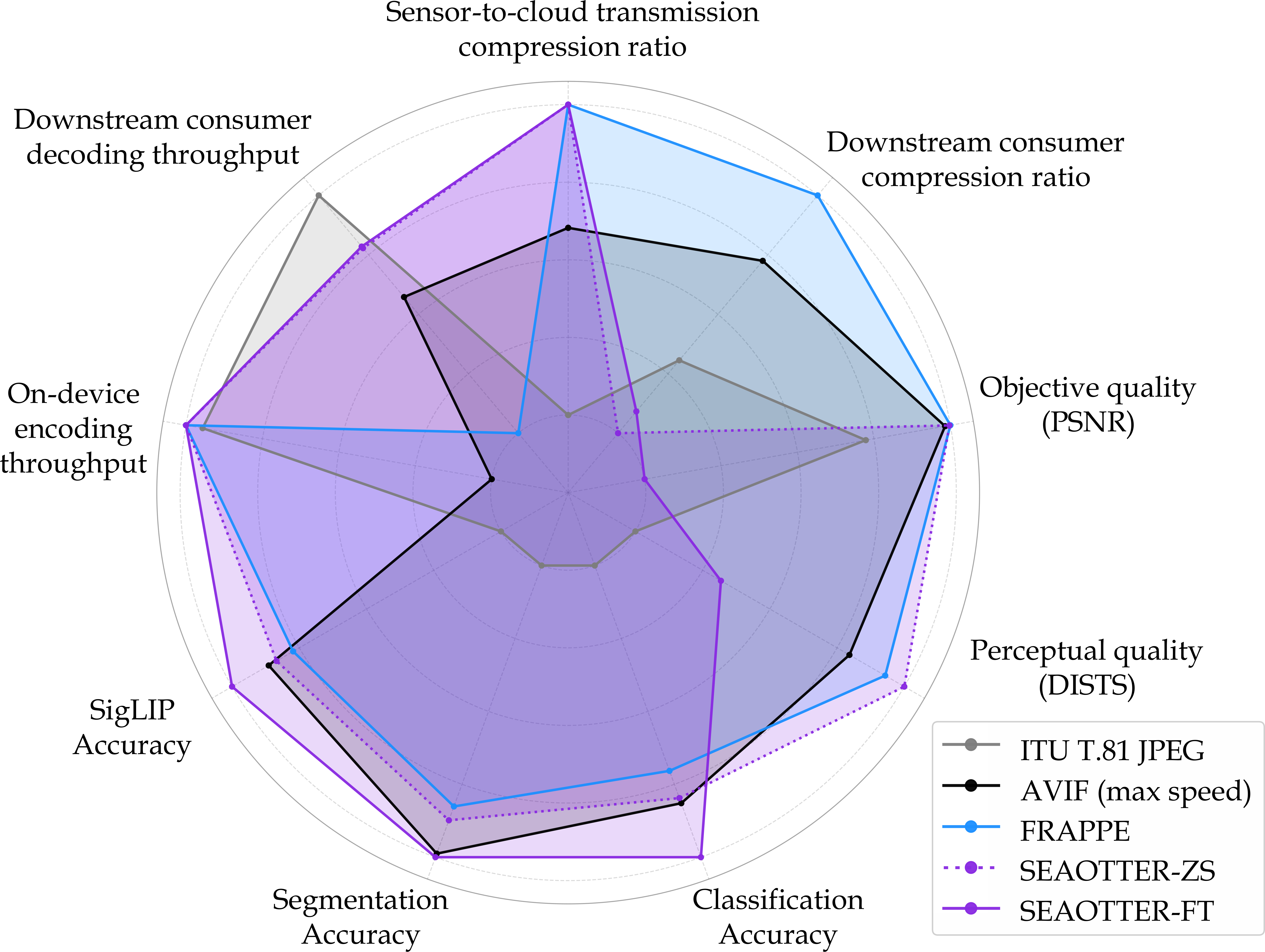
Fig. 28 Performance trade-offs of SEAOTTER variants vs other codecs.#
Transcode increases downstream accuracy. At matched transmit-bpp (\(0.109\), \(\text{CR}{=}221{:}1\)), SEAOTTER-FT achieves \(69.02\%\) ImageNet top-1 versus \(56.22\%\) for FRAPPE alone—a \(+12.80\) pp margin (Table 16). The gap widens at lower bitrates: at \(n{=}6\) (transmit-bpp \(0.038\)), SEAOTTER-FT reaches \(46.55\%\) where FRAPPE-only gives \(26.70\%\), a \(+19.85\) pp improvement. Even the zero-shot variant (SEAOTTER-ZS, no task-aware fine-tune) recovers \(+4.03\) pp over FRAPPE at \(n{=}12\). The same effect appears on ADE20K segmentation (mIoU \(+3.68\) pp for SEAOTTER-FT over FRAPPE at \(n{=}12\)) and SigLIP-2 zero-shot classification (top-1 \(+6.71\) pp).
Pareto dominance on machine-perception tasks. Under the matched-rate selection (Table 16; Fig. 29), SEAOTTER-FT leads ImageNet top-1 by \(+7.87\) pp over AVIF and \(+8.00\) pp over AVIF-max-speed, and leads SigLIP-2 zero-shot top-1 by \(+5.63\) pp and \(+4.03\) pp respectively—despite both baselines spending more bits per pixel. On ADE20K segmentation—the one axis where conventional baselines previously led at matched rate—SEAOTTER-FT now ties for first place (\(+0.02\) pp over AVIF, \(+0.26\) pp over AVIF-max-speed, \(+3.68\) pp over FRAPPE alone).
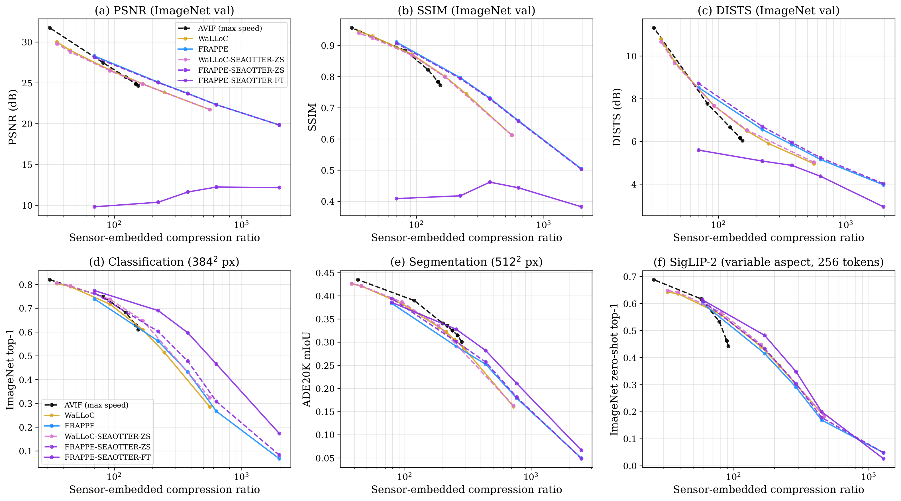
Fig. 29 Rate–distortion–accuracy trade-offs vs. transmit compression ratio: (top) SSIM and DISTS; (bottom) ADE20K mIoU and SigLIP-2 zero-shot top-1. SEAOTTER-ZS leads the perceptual-quality axes.#
Storage-side compression ratio. Figure 30 re-plots the three task accuracies against the storage compression ratio of the on-disk artifact. Against its architecturally-fair reference (FRAPPE followed by a vanilla ITU T.81 transcode at the same transmit-bpp), the SEAOTTER-FT artifact at \(n{=}12\) is \(13.7\%\) smaller and yields \(+8.19\) pp higher ImageNet top-1.
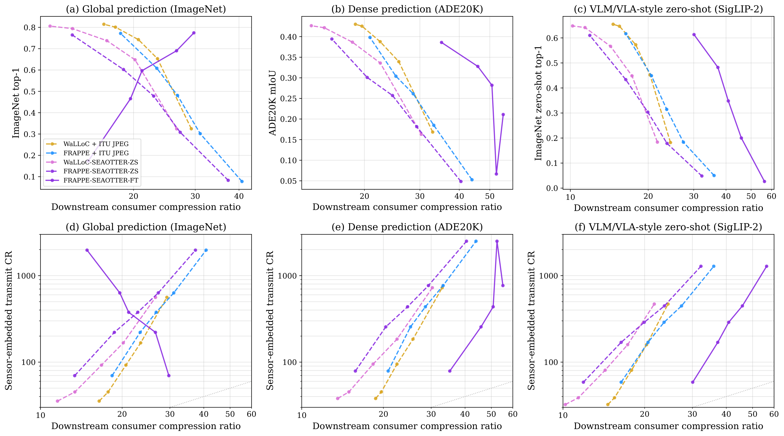
Fig. 30 Top row (a–c): downstream task accuracy vs. the storage compression ratio (on-disk JPEG size after transcode). Bottom row (d–f): sensor-embedded transmit CR vs. downstream consumer CR, with a \(y{=}x\) reference line.#
Sensor-side encoding throughput. All SEAOTTER variants inherit the same frozen FRAPPE encoder, so the sensor-side budget is identical to the FRAPPE-only baseline at every operating point (Table 16). At the per-task matched-rate ops the shared encoder is more than an order of magnitude faster than AVIF default-speed and \(5\)–\(8{\times}\) faster than AVIF max-speed across all three tasks, and exceeds \(250\) MPx/s for \(n{\le}9\)—sufficient for 1080p 30 fps over Wi-Fi after accounting for sensor-side concurrency (Fig. 25), with the SEAOTTER sandwich adding no encode-time overhead. Within-family encode differences (entries marked \(^{*}\) in Table 16) are measurement noise, not a real spread between the SEAOTTER-ZS and SEAOTTER-FT encoders.
Downstream consumer decoding throughput. The deployed steady-state consumer-side decode of a SEAOTTER artifact is a vanilla JPEG decode followed by \(\mathcal{F}^{-1}\). Measured end-to-end on CPU at \(384^2\) (Table 16, Throughput details), SEAOTTER’s consumer cost is therefore less than a third of AVIF’s decoding cost (\(\sim 3.4{\times}\) faster) and \(100{\times}\) faster than the same FRAPPE codec without the transcode. The advantage is structural: any consumer decodes the on-disk JPEG with ubiquitous standard hardware and may skip \(\mathcal{F}^{-1}\) altogether.
Deployment-tier suitability. We check whether each pipeline-and-op cell simultaneously clears three deployment-tier thresholds: BLE (\(\text{CR}{\ge}288\), encode \(\ge12\) MPx/s), 5G (\(\text{CR}{\ge}133\), encode \(\ge28\) MPx/s), and Wi-Fi (\(\text{CR}{\ge}60\), encode \(\ge62\) MPx/s). SEAOTTER-FT clears all three tiers at \(n\in\{3,6,9\}\) and the 5G and Wi-Fi tiers at \(n{=}12\) (missing only the BLE-tier CR by a thin margin); AVIF clears no tier at any quality we evaluate, and among the neural codecs WaLLoC clears only the BLE and 5G tiers at \(p{=}4\) (Table 23, Throughput details).
Why does the transcode help? The fine-tune deliberately drives reconstruction PSNR down (from \(25.08\) dB in vanilla FRAPPE to \(10.39\) dB in SEAOTTER-FT at \(n{=}12\); Per-task rate-distortion details) in exchange for downstream accuracy after the transcode. We hypothesize distribution calibration: the softsign companding and DCT-domain \(Q^{(k)}\) matrices push the consumer’s input back toward the standard JPEG distribution its JPEG-pretrained backbone expects, even where vanilla FRAPPE’s outputs look unlike any JPEG image.
Standalone learned JPEG vs ITU T.81 on Kodak#
To isolate the contribution of the learned JPEG sandwich without any FRAPPE-side encoding, we evaluate the trained \((\mathcal{F}, \mathcal{F}^{-1}, Q^{(0)}, Q^{(1)}, Q^{(2)})\) bundle as a standalone codec on the Kodak validation set (\(24\) images at native resolution: \(16\) images \(768{\times}512\), \(8\) images \(512{\times}768\); no resize, no crop) and compare against ITU T.81 with and without chroma subsampling. The \(7\)-step quality ladder for the ITU baselines is anchored to the three SEAOTTER operating points by choosing the smallest integer JPEG-sub\(=0\) quality at which SEAOTTER strictly dominates ITU T.81 4:4:4 on both Kodak PSNR and Kodak bpp, then interpolating intermediate q values. The learned sandwich strictly dominates ITU T.81 4:4:4 in PSNR at all three trained operating points, with margins of \(+0.27\) dB / \(+1.40\) dB / \(+1.27\) dB at matched bpp (Fig. 31 and Table 17). The standalone-codec evaluation establishes that the sandwich’s accuracy gain in the main paper is grounded in a learned representation that is also distortion-favourable in its own right, not a downstream-only artifact of the task-aware fine-tune.
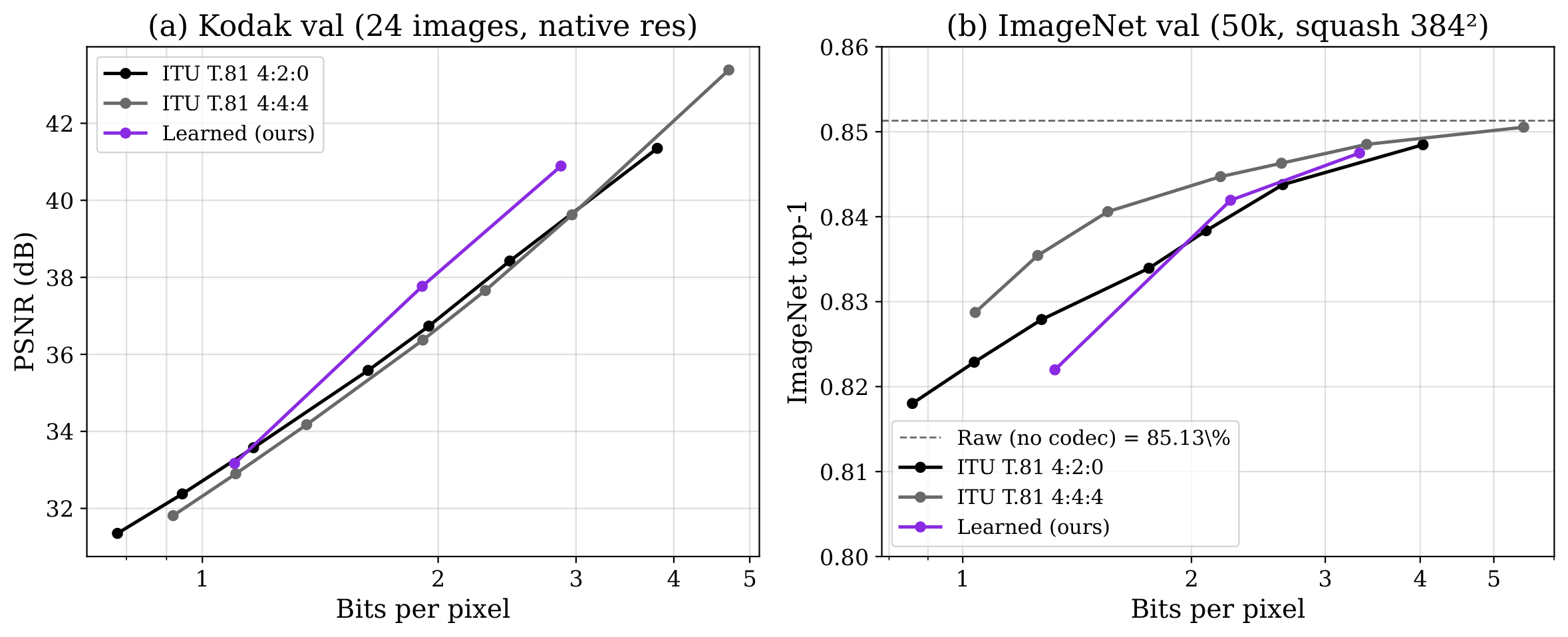
Fig. 31 Standalone learned JPEG codec versus ITU T.81 (with and without chroma subsampling) on the Kodak validation set at native resolution. SEAOTTER’s three trained operating points (\(k\in\{0,1,2\}\)) dominate matched-bpp ITU T.81 4:4:4 by \(+0.27\) / \(+1.40\) / \(+1.27\) dB in PSNR.#
Codec |
Setting |
bpp |
PSNR (dB) |
SSIM |
LPIPS (dB) |
DISTS (dB) |
|---|---|---|---|---|---|---|
ITU T.81 4:2:0 |
\(q=39\) |
0.779 |
31.35 |
0.952 |
5.93 |
13.15 |
ITU T.81 4:2:0 |
\(q=53\) |
0.943 |
32.38 |
0.963 |
6.68 |
14.56 |
ITU T.81 4:2:0 |
\(q=67\) |
1.162 |
33.58 |
0.972 |
7.54 |
16.07 |
ITU T.81 4:2:0 |
\(q=81\) |
1.628 |
35.58 |
0.982 |
9.11 |
18.67 |
ITU T.81 4:2:0 |
\(q=86\) |
1.946 |
36.73 |
0.985 |
10.05 |
20.12 |
ITU T.81 4:2:0 |
\(q=91\) |
2.469 |
38.42 |
0.989 |
11.51 |
21.71 |
ITU T.81 4:2:0 |
\(q=96\) |
3.810 |
41.35 |
0.993 |
14.60 |
23.94 |
ITU T.81 4:4:4 |
\(q=39\) |
0.917 |
31.81 |
0.958 |
6.30 |
15.16 |
ITU T.81 4:4:4 |
\(q=53\) |
1.103 |
32.90 |
0.969 |
7.14 |
16.90 |
ITU T.81 4:4:4 |
\(q=67\) |
1.359 |
34.17 |
0.978 |
8.08 |
18.65 |
ITU T.81 4:4:4 |
\(q=81\) |
1.912 |
36.37 |
0.987 |
9.85 |
22.08 |
ITU T.81 4:4:4 |
\(q=86\) |
2.298 |
37.66 |
0.991 |
10.90 |
23.97 |
ITU T.81 4:4:4 |
\(q=91\) |
2.965 |
39.62 |
0.994 |
12.60 |
25.83 |
ITU T.81 4:4:4 |
\(q=96\) |
4.701 |
43.38 |
0.997 |
16.36 |
28.39 |
SEAOTTER (ours) |
\(k=0\) |
1.099 |
33.17 |
0.943 |
6.00 |
12.44 |
SEAOTTER (ours) |
\(k=1\) |
1.909 |
37.77 |
0.980 |
9.42 |
17.55 |
SEAOTTER (ours) |
\(k=2\) |
2.870 |
40.89 |
0.991 |
12.85 |
21.61 |
Standalone learned JPEG on ImageNet#
Table 18 re-evaluates the same \(17\) standalone-codec cells on ImageNet val (\(50{,}000\) images, squash-\(384^2\) preprocessing, the same teacher as the main classification task) and reports top-1 accuracy plus PSNR. The standalone sandwich is evaluated without the FRAPPE-side upstream that the main paper’s SEAOTTER pipeline uses.
Codec |
Setting |
bpp |
Top-1 (%) |
PSNR (dB) |
|---|---|---|---|---|
ITU T.81 4:2:0 |
\(q=39\) |
0.858 |
81.80 |
30.39 |
ITU T.81 4:2:0 |
\(q=53\) |
1.036 |
82.29 |
31.29 |
ITU T.81 4:2:0 |
\(q=67\) |
1.270 |
82.79 |
32.35 |
ITU T.81 4:2:0 |
\(q=81\) |
1.758 |
83.39 |
34.09 |
ITU T.81 4:2:0 |
\(q=86\) |
2.091 |
83.84 |
35.06 |
ITU T.81 4:2:0 |
\(q=91\) |
2.638 |
84.38 |
36.42 |
ITU T.81 4:2:0 |
\(q=96\) |
4.034 |
84.85 |
38.62 |
ITU T.81 4:4:4 |
\(q=39\) |
1.039 |
82.87 |
31.12 |
ITU T.81 4:4:4 |
\(q=53\) |
1.255 |
83.54 |
32.14 |
ITU T.81 4:4:4 |
\(q=67\) |
1.552 |
84.06 |
33.38 |
ITU T.81 4:4:4 |
\(q=81\) |
2.184 |
84.47 |
35.50 |
ITU T.81 4:4:4 |
\(q=86\) |
2.627 |
84.63 |
36.74 |
ITU T.81 4:4:4 |
\(q=91\) |
3.401 |
84.85 |
38.65 |
ITU T.81 4:4:4 |
\(q=96\) |
5.473 |
85.05 |
42.61 |
SEAOTTER (ours) |
\(k=0\) |
1.322 |
82.20 |
32.50 |
SEAOTTER (ours) |
\(k=1\) |
2.252 |
84.19 |
36.56 |
SEAOTTER (ours) |
\(k=2\) |
3.328 |
84.75 |
39.07 |
Per-task rate-distortion details#
Tables 19–21 report per-pipeline per-op detail for the three downstream tasks (cls / seg / clip). Each table reports both the transmit bpp (the sensor-uplink rate) and the storage bpp (the on-disk JPEG file after the cloud-side transcode); for codecs without a transcode step the two values coincide. The raw row is the no-codec ceiling for context. SEAOTTER-FT’s reconstruction PSNR is intentionally low because the fine-tune trades pixel fidelity for downstream accuracy (Accuracy Gains from Negative-Distortion Transcoding); we report PSNR for transparency, not as a quality target.
Pipeline |
Op |
Transmit bpp |
Storage bpp |
Top-1 (%) |
PSNR (dB) |
|---|---|---|---|---|---|
AVIF |
\(q=1\) |
0.1458 |
0.1458 |
61.15 |
25.01 |
\(q=5\) |
0.1525 |
0.1525 |
62.70 |
25.24 |
|
\(q=6\) |
0.1628 |
0.1628 |
64.67 |
25.56 |
|
\(q=10\) |
0.1840 |
0.1840 |
68.11 |
26.17 |
|
\(q=25\) |
0.2756 |
0.2756 |
75.53 |
27.95 |
|
\(q=50\) |
0.7100 |
0.7100 |
82.09 |
32.28 |
|
AVIF (max-speed) |
\(q=1\) |
0.1558 |
0.1558 |
61.02 |
24.65 |
\(q=3\) |
0.1624 |
0.1624 |
62.80 |
24.85 |
|
\(q=5\) |
0.1624 |
0.1624 |
62.80 |
24.85 |
|
\(q=10\) |
0.1948 |
0.1948 |
68.22 |
25.70 |
|
\(q=25\) |
0.2934 |
0.2934 |
74.87 |
27.46 |
|
\(q=50\) |
0.7730 |
0.7730 |
82.01 |
31.75 |
|
FRAPPE |
\(n=3\) |
0.0122 |
0.0122 |
6.77 |
19.85 |
\(n=6\) |
0.0380 |
0.0380 |
26.70 |
22.34 |
|
\(n=9\) |
0.0637 |
0.0637 |
43.21 |
23.71 |
|
\(n=12\) |
0.1086 |
0.1086 |
56.22 |
25.08 |
|
\(n=15\) |
0.3439 |
0.3439 |
73.91 |
28.29 |
|
WaLLoC |
\(p=4\) |
0.0428 |
0.0428 |
28.56 |
21.74 |
\(p=10.5\) |
0.0971 |
0.0971 |
51.40 |
23.84 |
|
\(p=16\) |
0.1437 |
0.1437 |
60.98 |
24.88 |
|
\(p=36\) |
0.2598 |
0.2598 |
71.70 |
26.57 |
|
\(p=80\) |
0.5312 |
0.5312 |
79.10 |
28.97 |
|
\(p=100\) |
0.6773 |
0.6773 |
80.40 |
30.01 |
|
SEAOTTER-ZS |
\(n=3\) |
0.0122 |
0.6441 |
8.30 |
19.84 |
\(n=6\) |
0.0380 |
0.8829 |
30.81 |
22.32 |
|
\(n=9\) |
0.0637 |
1.0510 |
47.78 |
23.69 |
|
\(n=12\) |
0.1086 |
1.2822 |
60.25 |
25.04 |
|
\(n=15\) |
0.3439 |
1.7950 |
76.43 |
28.16 |
|
WaLLoC-SEAOTTER-ZS |
\(p=4\) |
0.0428 |
0.9038 |
32.42 |
21.73 |
\(p=16\) |
0.1437 |
1.1884 |
64.80 |
24.84 |
|
\(p=36\) |
0.2598 |
1.4300 |
73.76 |
26.49 |
|
\(p=80\) |
0.5312 |
1.7925 |
79.41 |
28.79 |
|
\(p=100\) |
0.6773 |
2.0772 |
80.59 |
29.79 |
|
SEAOTTER-FT |
\(n=3\) |
0.0122 |
1.6163 |
17.34 |
12.18 |
\(n=6\) |
0.0380 |
1.2243 |
46.55 |
12.25 |
|
\(n=9\) |
0.0637 |
1.1352 |
59.69 |
11.64 |
|
\(n=12\) |
0.1086 |
0.9046 |
69.02 |
10.39 |
|
\(n=15\) |
0.3439 |
0.8073 |
77.43 |
9.83 |
|
Raw (no codec) |
– |
14.6658 |
14.6658 |
85.13 |
120.00 |
Pipeline |
Op |
Transmit bpp |
Storage bpp |
mIoU (%) |
PSNR (dB) |
|---|---|---|---|---|---|
AVIF |
\(q=1\) |
0.0794 |
0.0794 |
30.85 |
26.67 |
\(q=5\) |
0.0860 |
0.0860 |
32.75 |
26.97 |
|
\(q=6\) |
0.0945 |
0.0945 |
33.43 |
27.36 |
|
\(q=10\) |
0.1117 |
0.1117 |
35.27 |
28.09 |
|
\(q=25\) |
0.1850 |
0.1850 |
39.46 |
30.28 |
|
\(q=50\) |
0.5103 |
0.5103 |
43.37 |
35.65 |
|
AVIF (max-speed) |
\(q=1\) |
0.0851 |
0.0851 |
30.06 |
26.29 |
\(q=3\) |
0.0918 |
0.0918 |
31.47 |
26.56 |
|
\(q=5\) |
0.0918 |
0.0918 |
31.47 |
26.56 |
|
\(q=6\) |
0.1007 |
0.1007 |
32.51 |
26.93 |
|
\(q=7\) |
0.1007 |
0.1007 |
32.51 |
26.93 |
|
\(q=8\) |
0.1106 |
0.1106 |
33.56 |
27.31 |
|
\(q=9\) |
0.1106 |
0.1106 |
33.56 |
27.31 |
|
\(q=10\) |
0.1197 |
0.1197 |
34.05 |
27.63 |
|
\(q=25\) |
0.2021 |
0.2021 |
38.99 |
29.89 |
|
\(q=50\) |
0.5648 |
0.5648 |
43.49 |
35.12 |
|
FRAPPE |
\(n=3\) |
0.0096 |
0.0096 |
4.95 |
20.70 |
\(n=6\) |
0.0312 |
0.0312 |
17.91 |
23.52 |
|
\(n=9\) |
0.0550 |
0.0550 |
25.24 |
25.14 |
|
\(n=12\) |
0.0939 |
0.0939 |
29.09 |
26.81 |
|
\(n=15\) |
0.3042 |
0.3042 |
38.38 |
30.48 |
|
WaLLoC |
\(p=4\) |
0.0331 |
0.0331 |
16.07 |
22.64 |
\(p=10.5\) |
0.0817 |
0.0817 |
28.72 |
25.13 |
|
\(p=11\) |
0.0968 |
0.0968 |
30.51 |
25.64 |
|
\(p=12\) |
0.0968 |
0.0968 |
30.51 |
25.64 |
|
\(p=13\) |
0.1127 |
0.1127 |
32.21 |
26.13 |
|
\(p=14\) |
0.1127 |
0.1127 |
32.21 |
26.13 |
|
\(p=15\) |
0.1127 |
0.1127 |
32.21 |
26.13 |
|
\(p=16\) |
0.1300 |
0.1300 |
33.31 |
26.58 |
|
\(p=36\) |
0.2531 |
0.2531 |
38.33 |
28.98 |
|
\(p=80\) |
0.5306 |
0.5306 |
42.12 |
32.07 |
|
\(p=100\) |
0.6320 |
0.6320 |
42.60 |
32.96 |
|
SEAOTTER-ZS |
\(n=3\) |
0.0096 |
0.5928 |
4.84 |
20.69 |
\(n=6\) |
0.0312 |
0.8188 |
18.15 |
23.51 |
|
\(n=9\) |
0.0550 |
0.9773 |
25.71 |
25.12 |
|
\(n=12\) |
0.0939 |
1.1759 |
30.09 |
26.77 |
|
\(n=15\) |
0.3042 |
1.5222 |
39.42 |
30.37 |
|
WaLLoC-SEAOTTER-ZS |
\(p=4\) |
0.0331 |
0.7921 |
16.28 |
22.63 |
\(p=16\) |
0.1300 |
1.0685 |
33.58 |
26.54 |
|
\(p=36\) |
0.2531 |
1.3098 |
38.66 |
28.88 |
|
\(p=80\) |
0.5306 |
1.6084 |
42.16 |
31.85 |
|
\(p=100\) |
0.6320 |
1.7689 |
42.65 |
32.74 |
|
SEAOTTER-FT |
\(n=3\) |
0.0096 |
0.4575 |
6.66 |
10.13 |
\(n=6\) |
0.0312 |
0.4352 |
21.10 |
10.55 |
|
\(n=9\) |
0.0550 |
0.4726 |
28.20 |
10.78 |
|
\(n=12\) |
0.0939 |
0.5240 |
32.77 |
10.76 |
|
\(n=15\) |
0.3042 |
0.6830 |
38.59 |
12.21 |
|
Raw (no codec) |
– |
11.1280 |
11.1280 |
44.51 |
120.00 |
Pipeline |
Op |
Transmit bpp |
Storage bpp |
Zero-shot Top-1 (%) |
PSNR (dB) |
|---|---|---|---|---|---|
AVIF |
\(q=1\) |
0.2503 |
0.2503 |
42.59 |
24.34 |
\(q=5\) |
0.2581 |
0.2581 |
44.84 |
24.57 |
|
\(q=6\) |
0.2701 |
0.2701 |
47.98 |
24.91 |
|
\(q=10\) |
0.2941 |
0.2941 |
52.17 |
25.52 |
|
\(q=25\) |
0.3963 |
0.3963 |
61.08 |
27.32 |
|
\(q=50\) |
0.8698 |
0.8698 |
68.67 |
31.66 |
|
AVIF (max-speed) |
\(q=1\) |
0.2633 |
0.2633 |
44.19 |
23.96 |
\(q=3\) |
0.2709 |
0.2709 |
46.24 |
24.16 |
|
\(q=5\) |
0.2709 |
0.2709 |
46.24 |
24.16 |
|
\(q=10\) |
0.3073 |
0.3073 |
53.29 |
25.02 |
|
\(q=25\) |
0.4169 |
0.4169 |
61.67 |
26.78 |
|
\(q=50\) |
0.9389 |
0.9389 |
68.80 |
31.05 |
|
FRAPPE |
\(n=3\) |
0.0187 |
0.0187 |
4.84 |
18.91 |
\(n=6\) |
0.0537 |
0.0537 |
16.94 |
21.50 |
|
\(n=9\) |
0.0831 |
0.0831 |
29.03 |
22.92 |
|
\(n=12\) |
0.1417 |
0.1417 |
41.51 |
24.37 |
|
\(n=15\) |
0.4095 |
0.4095 |
60.13 |
27.68 |
|
WaLLoC |
\(p=4\) |
0.0511 |
0.0511 |
18.23 |
20.30 |
\(p=10.5\) |
0.1101 |
0.1101 |
36.95 |
22.72 |
|
\(p=16\) |
0.1508 |
0.1508 |
44.05 |
23.66 |
|
\(p=36\) |
0.2973 |
0.2973 |
55.85 |
25.81 |
|
\(p=80\) |
0.6195 |
0.6195 |
63.62 |
28.58 |
|
\(p=100\) |
0.7422 |
0.7422 |
64.24 |
29.48 |
|
SEAOTTER-ZS |
\(n=3\) |
0.0187 |
0.7441 |
4.84 |
18.90 |
\(n=6\) |
0.0537 |
1.0148 |
17.87 |
21.49 |
|
\(n=9\) |
0.0831 |
1.2040 |
30.36 |
22.90 |
|
\(n=12\) |
0.1417 |
1.4650 |
43.34 |
24.32 |
|
\(n=15\) |
0.4095 |
2.0182 |
61.00 |
27.54 |
|
WaLLoC-SEAOTTER-ZS |
\(p=4\) |
0.0511 |
1.1057 |
18.37 |
20.30 |
\(p=16\) |
0.1508 |
1.3863 |
44.85 |
23.64 |
|
\(p=36\) |
0.2973 |
1.6776 |
56.65 |
25.75 |
|
\(p=80\) |
0.6195 |
2.1065 |
64.14 |
28.39 |
|
\(p=100\) |
0.7422 |
2.3531 |
64.78 |
29.26 |
|
SEAOTTER-FT |
\(n=3\) |
0.0187 |
0.4261 |
2.65 |
9.47 |
\(n=6\) |
0.0537 |
0.5235 |
20.01 |
12.68 |
|
\(n=9\) |
0.0831 |
0.5879 |
34.82 |
13.43 |
|
\(n=12\) |
0.1417 |
0.6451 |
48.22 |
13.07 |
|
\(n=15\) |
0.4095 |
0.7980 |
61.34 |
12.78 |
|
Raw (no codec) |
– |
15.1991 |
15.1991 |
69.59 |
120.00 |
Throughput details#
Table 22 reports wall-clock measurements for sensor-side encode and steady-state consumer-side codec decode (no downstream teacher forward) per pipeline-and-op for the cls task. Each row reports the median over a \(32\)-image distribution at batch size \(1\) on an AMD EPYC 9354 CPU. For SEAOTTER-family pipelines (SEAOTTER-ZS / SEAOTTER-FT / their WaLLoC-side counterparts) the decode column is the deployed consumer cost: a vanilla JPEG decode followed by the \(3{\times}3\) inverse-conv \(\mathcal{F}^{-1}\) and per-channel companding. The one-time cloud-side transcode (FRAPPE/WaLLoC neural decode \(\to\) sandwich forward \(\to\) JPEG encode) is paid once per image and not counted in the decode column; it has the same wall-clock as the corresponding FRAPPE-only / WaLLoC-only row’s decode.
Pipeline |
Op |
Transmit bpp |
Enc. (ms) |
Dec. (ms) |
Enc. (MPx/s) |
Dec. (MPx/s) |
|---|---|---|---|---|---|---|
AVIF (default) |
\(q=1\) |
0.1458 |
26.75 |
7.47 |
5.51 |
19.75 |
\(q=5\) |
0.1525 |
28.40 |
7.45 |
5.19 |
19.79 |
|
\(q=6\) |
0.1628 |
28.67 |
7.42 |
5.14 |
19.87 |
|
\(q=10\) |
0.1840 |
31.99 |
7.56 |
4.61 |
19.50 |
|
\(q=25\) |
0.2756 |
38.09 |
7.72 |
3.87 |
19.10 |
|
\(q=50\) |
0.7100 |
52.63 |
7.92 |
2.80 |
18.62 |
|
AVIF (max speed) |
\(q=1\) |
0.1558 |
5.73 |
7.55 |
25.73 |
19.53 |
\(q=3\) |
0.1624 |
5.75 |
7.55 |
25.66 |
19.54 |
|
\(q=5\) |
0.1624 |
5.77 |
8.06 |
25.55 |
18.29 |
|
\(q=10\) |
0.1948 |
5.91 |
7.97 |
24.97 |
18.49 |
|
\(q=25\) |
0.2934 |
6.42 |
8.24 |
22.96 |
17.90 |
|
\(q=50\) |
0.7730 |
8.12 |
8.05 |
18.15 |
18.31 |
|
FRAPPE |
\(n=3\) |
0.0122 |
0.25 |
223.72 |
601.47\(^{*}\) |
0.66 |
\(n=6\) |
0.0380 |
0.46 |
236.76 |
317.23\(^{*}\) |
0.62 |
|
\(n=9\) |
0.0637 |
0.54 |
212.46 |
271.81\(^{*}\) |
0.69 |
|
\(n=12\) |
0.1086 |
0.83 |
218.06 |
177.76\(^{*}\) |
0.68 |
|
\(n=15\) |
0.3439 |
1.36 |
214.20 |
108.17\(^{*}\) |
0.69 |
|
WaLLoC |
\(p=4\) |
0.0428 |
2.59 |
113.77 |
57.00\(^{*}\) |
1.30 |
\(p=10.5\) |
0.0971 |
3.76 |
45.20 |
39.26\(^{*}\) |
3.26 |
|
\(p=16\) |
0.1437 |
4.89 |
37.43 |
30.17\(^{*}\) |
3.94 |
|
\(p=36\) |
0.2598 |
7.82 |
67.26 |
18.85\(^{*}\) |
2.19 |
|
\(p=80\) |
0.5312 |
13.37 |
131.60 |
11.03\(^{*}\) |
1.12 |
|
\(p=100\) |
0.6773 |
13.17 |
135.77 |
11.20\(^{*}\) |
1.09 |
|
SEAOTTER-ZS |
\(n=3\) |
0.0122 |
0.25 |
2.14 |
601.47\(^{*}\) |
68.82 |
\(n=6\) |
0.0380 |
0.46 |
2.24 |
317.23\(^{*}\) |
65.72 |
|
\(n=9\) |
0.0637 |
0.54 |
2.77 |
271.81\(^{*}\) |
53.14 |
|
\(n=12\) |
0.1086 |
0.83 |
2.26 |
177.76\(^{*}\) |
65.35 |
|
\(n=15\) |
0.3439 |
1.36 |
2.71 |
108.17\(^{*}\) |
54.49 |
|
SEAOTTER-ZS (WaLLoC encode) |
\(p=4\) |
0.0428 |
2.59 |
3.18 |
57.00\(^{*}\) |
46.39 |
\(p=16\) |
0.1437 |
4.89 |
2.92 |
30.17\(^{*}\) |
50.58 |
|
\(p=36\) |
0.2598 |
7.82 |
2.90 |
18.85\(^{*}\) |
50.80 |
|
\(p=80\) |
0.5312 |
13.37 |
2.21 |
11.03\(^{*}\) |
66.71 |
|
\(p=100\) |
0.6773 |
13.17 |
3.08 |
11.20\(^{*}\) |
47.88 |
|
SEAOTTER-FT |
\(n=3\) |
0.0122 |
0.25 |
2.19 |
601.47\(^{*}\) |
67.30 |
\(n=6\) |
0.0380 |
0.46 |
2.32 |
317.23\(^{*}\) |
63.59 |
|
\(n=9\) |
0.0637 |
0.54 |
2.51 |
271.81\(^{*}\) |
58.83 |
|
\(n=12\) |
0.1086 |
0.83 |
2.17 |
177.76\(^{*}\) |
67.97 |
|
\(n=15\) |
0.3439 |
1.36 |
2.34 |
108.17\(^{*}\) |
62.94 |
Conventional-codec configuration.
All conventional-codec timings use Pillow 12.2: JPEG is encoded and decoded through libjpeg-turbo, and AVIF through Pillow’s built-in libavif (libaom for encoding, dav1d for decoding); no pillow-avif-plugin and no GPU or hardware-codec acceleration are involved. Quality is set by Pillow’s quality parameter, and the AVIF max-speed variant adds speed=10. AVIF uses libavif’s default \(4{:}2{:}0\) chroma subsampling; the main-table JPEG likewise uses \(4{:}2{:}0\), while the standalone-codec comparison (Standalone learned JPEG vs ITU T.81 on Kodak) uses \(4{:}4{:}4\) (subsampling=0). All measurements run in a single Python process at batch size \(1\) on one AMD EPYC 9354 CPU; the harness requests no explicit multi-threading, so each backend runs at its library default with SIMD enabled. Neural encoders run under torch.inference_mode(). Following the FRAPPE reference harness, each stage is timed with n_warmup\(=1\) and n_measurement\(=5\) (median per stage), reproducing the reference to within \({\sim}1\)–\(3\%\).
Table 23 reports, for every pipeline-and-op cell in the comparison, whether the cell simultaneously clears each of the three deployment-tier thresholds defined in Accuracy Gains from Negative-Distortion Transcoding. SEAOTTER and FRAPPE clear all three tiers at low-bitrate operating points; AVIF clears no tier at any quality we evaluate.
Pipeline |
Op |
Transmit CR |
Encode (MPx/s) |
BLE |
5G |
Wi-Fi |
|---|---|---|---|---|---|---|
FRAPPE |
\(n=3\) |
1972.6:1 |
601.47 |
✓ |
✓ |
✓ |
SEAOTTER-ZS |
\(n=3\) |
1972.6:1 |
601.47 |
✓ |
✓ |
✓ |
SEAOTTER-FT |
\(n=3\) |
1972.6:1 |
601.47 |
✓ |
✓ |
✓ |
FRAPPE |
\(n=6\) |
632.2:1 |
317.23 |
✓ |
✓ |
✓ |
SEAOTTER-ZS |
\(n=6\) |
632.2:1 |
317.23 |
✓ |
✓ |
✓ |
SEAOTTER-FT |
\(n=6\) |
632.2:1 |
317.23 |
✓ |
✓ |
✓ |
WaLLoC |
\(p=4\) |
561.2:1 |
57.00 |
✓ |
✓ |
\(\cdot\) |
WaLLoC-SEAOTTER-ZS |
\(p=4\) |
561.2:1 |
57.00 |
✓ |
✓ |
\(\cdot\) |
FRAPPE |
\(n=9\) |
376.9:1 |
271.81 |
✓ |
✓ |
✓ |
SEAOTTER-ZS |
\(n=9\) |
376.9:1 |
271.81 |
✓ |
✓ |
✓ |
SEAOTTER-FT |
\(n=9\) |
376.9:1 |
271.81 |
✓ |
✓ |
✓ |
WaLLoC |
\(p=10.5\) |
247.1:1 |
39.26 |
\(\cdot\) |
✓ |
\(\cdot\) |
FRAPPE |
\(n=12\) |
221.0:1 |
177.76 |
\(\cdot\) |
✓ |
✓ |
SEAOTTER-ZS |
\(n=12\) |
221.0:1 |
177.76 |
\(\cdot\) |
✓ |
✓ |
SEAOTTER-FT |
\(n=12\) |
221.0:1 |
177.76 |
\(\cdot\) |
✓ |
✓ |
WaLLoC |
\(p=16\) |
167.0:1 |
30.17 |
\(\cdot\) |
✓ |
\(\cdot\) |
WaLLoC-SEAOTTER-ZS |
\(p=16\) |
167.0:1 |
30.17 |
\(\cdot\) |
✓ |
\(\cdot\) |
AVIF |
\(q=1\) |
164.6:1 |
5.51 |
\(\cdot\) |
\(\cdot\) |
\(\cdot\) |
AVIF |
\(q=5\) |
157.4:1 |
5.19 |
\(\cdot\) |
\(\cdot\) |
\(\cdot\) |
AVIF (max-speed) |
\(q=1\) |
154.1:1 |
25.73 |
\(\cdot\) |
\(\cdot\) |
\(\cdot\) |
AVIF (max-speed) |
\(q=3\) |
147.7:1 |
25.66 |
\(\cdot\) |
\(\cdot\) |
\(\cdot\) |
AVIF (max-speed) |
\(q=5\) |
147.7:1 |
25.55 |
\(\cdot\) |
\(\cdot\) |
\(\cdot\) |
AVIF |
\(q=6\) |
147.4:1 |
5.14 |
\(\cdot\) |
\(\cdot\) |
\(\cdot\) |
AVIF |
\(q=10\) |
130.4:1 |
4.61 |
\(\cdot\) |
\(\cdot\) |
\(\cdot\) |
AVIF (max-speed) |
\(q=10\) |
123.2:1 |
24.97 |
\(\cdot\) |
\(\cdot\) |
\(\cdot\) |
WaLLoC |
\(p=36\) |
92.4:1 |
18.85 |
\(\cdot\) |
\(\cdot\) |
\(\cdot\) |
WaLLoC-SEAOTTER-ZS |
\(p=36\) |
92.4:1 |
18.85 |
\(\cdot\) |
\(\cdot\) |
\(\cdot\) |
AVIF |
\(q=25\) |
87.1:1 |
3.87 |
\(\cdot\) |
\(\cdot\) |
\(\cdot\) |
AVIF (max-speed) |
\(q=25\) |
81.8:1 |
22.96 |
\(\cdot\) |
\(\cdot\) |
\(\cdot\) |
FRAPPE |
\(n=15\) |
69.8:1 |
108.17 |
\(\cdot\) |
\(\cdot\) |
✓ |
SEAOTTER-ZS |
\(n=15\) |
69.8:1 |
108.17 |
\(\cdot\) |
\(\cdot\) |
✓ |
SEAOTTER-FT |
\(n=15\) |
69.8:1 |
108.17 |
\(\cdot\) |
\(\cdot\) |
✓ |
WaLLoC |
\(p=80\) |
45.2:1 |
11.03 |
\(\cdot\) |
\(\cdot\) |
\(\cdot\) |
WaLLoC-SEAOTTER-ZS |
\(p=80\) |
45.2:1 |
11.03 |
\(\cdot\) |
\(\cdot\) |
\(\cdot\) |
WaLLoC |
\(p=100\) |
35.4:1 |
11.20 |
\(\cdot\) |
\(\cdot\) |
\(\cdot\) |
WaLLoC-SEAOTTER-ZS |
\(p=100\) |
35.4:1 |
11.20 |
\(\cdot\) |
\(\cdot\) |
\(\cdot\) |
AVIF |
\(q=50\) |
33.8:1 |
2.80 |
\(\cdot\) |
\(\cdot\) |
\(\cdot\) |
AVIF (max-speed) |
\(q=50\) |
31.0:1 |
18.15 |
\(\cdot\) |
\(\cdot\) |
\(\cdot\) |
Training recipe#
For our headline \(K{=}3\) configuration we use Lagrange multipliers \((\lambda_1, \lambda_2, \lambda_3) = (0.75, 0.40, 0.22)\) and per-rate loss weights \((w_1, w_2, w_3) = (0.3, 0.7, 1.5)\). Training is performed on the LSDIR dataset (Li et al., 2023) at \(480^2\) crops for \(4\) epochs, using the Adan optimizer (Xie et al., 2024) (with caution=True), a raised-cosine learning-rate schedule with base learning rate \(1.2{\times}10^{-2}\) (the qtable parameter group runs at half the base rate), batch size \(4\) per GPU on \(4{\times}\) RTX PRO 6000 GPUs, gradient clipping at \(5.0\), and seed \(0\). The trained \((\mathcal{F}, \mathcal{F}^{-1})\) pair, the three \(Q^{(k)}\) matrices, and the three calibrated rate-proxy scalars are bundled together and published as a single artifact loaded by every downstream experiment via a single library call.
Experiment details#
The cls teacher checkpoint is convnext_tiny.in12k_ft_in1k_384; its no-codec ceiling on this teacher and protocol is \(85.13\%\) top-1. The seg no-codec ceiling under the squash-\(512^2\) protocol is \(44.51\%\) mIoU (about \(1.5\) pp below the sliding-window paper-protocol number for the same teacher). The clip naflex preprocessing uses max_num_patches\(=256\), patch_size\(=16\), snap\(=32\); its no-codec ceiling is \(69.59\%\) zero-shot top-1. All wall-clock timings are measured at batch size \(1\) on an AMD EPYC 9354 CPU paired with an RTX PRO 6000 Blackwell Max-Q GPU.
Conclusion#
We presented SEAOTTER, a compression framework for cloud robotics that pairs a sensor-embedded autoencoder with a one-time cloud-side transcode into a standards-compliant JPEG file. Across global, dense, and zero-shot perception, the transcode increases downstream accuracy over the same DNN-based autoencoder used without it, while producing on-disk artifacts that virtually any data consumer can use.
Limitations and future work. (i) Modality coverage. We test only RGB; depth, IR, multispectral, and hyperspectral signals are a natural extension the framework handles without architectural changes but that we have not characterized. (ii) Component ablations. We do not isolate the contributions of the softsign companding, the DCT-domain \(Q^{(k)}\) matrices, and the \(3{\times}3\) wrapper filter. (iii) Sensor / lighting variation. How the learned (approximately YCgCo) color transform varies across sensors, lighting, and lens distortions—and whether per-domain \(\mathcal{F}\) pairs help—is left to future work. (iv) Human perception. We have not evaluated human perception (e.g., teleoperation) of SEAOTTER-JPEG artifacts versus standard JPEG/AVIF at matched storage rate—important given the nonstandard color space.
References#
Niranjan Balasubramanian, Aruna Balasubramanian, and Arun Venkataramani. Energy consumption in mobile phones: a measurement study and implications for network applications. In Proceedings of the 9th ACM SIGCOMM Conference on Internet Measurement, 280–293. 2009.
Johannes Ballé, Valero Laparra, and Eero P. Simoncelli. End-to-end optimized image compression. In International Conference on Learning Representations. 2017. URL: https://openreview.net/forum?id=rJxdQ3jeg.
Johannes Ballé, David Minnen, Saurabh Singh, Sung Jin Hwang, and Nick Johnston. Variational image compression with a scale hyperprior. ICML, 2018.
Lucas Beyer. On the speed of ViTs and CNNs. http://lb.eyer.be/a/vit-cnn-speed.html, 2024.
Frank Bossen, Karsten Sühring, Adam Wieckowski, and Shan Liu. VVC complexity and software implementation analysis. IEEE Transactions on Circuits and Systems for Video Technology, 31(10):3765–3778, 2021.
Aaron Carroll and Gernot Heiser. An analysis of power consumption in a smartphone. In 2010 USENIX Annual Technical Conference (USENIX ATC 10). 2010.
Denis Guangyin Chen, Fang Tang, Man-Kay Law, and Amine Bermak. A 12 pj/pixel analog-to-information converter based 816× 640 pixel cmos image sensor. IEEE Journal of Solid-State Circuits, 49(5):1210–1222, 2014.
Jia Deng, Wei Dong, Richard Socher, Li-Jia Li, Kai Li, and Li Fei-Fei. Imagenet: a large-scale hierarchical image database. In CVPR. 2009.
Keyan Ding, Keda Ma, Shiqi Wang, and Eero P Simoncelli. Image quality assessment: unifying structure and texture similarity. IEEE transactions on pattern analysis and machine intelligence, 2020.
Max Ehrlich and Larry S Davis. Deep residual learning in the jpeg transform domain. In ICCV. 2019.
Changsheng Gao, Yifan Ma, Qiaoxi Chen, Yenan Xu, Dong Liu, and Weisi Lin. Feature coding in the era of large models: dataset, test conditions, and benchmark. In Proceedings of the IEEE/CVF International Conference on Computer Vision, 1068–1077. 2025.
Lionel Gueguen, Alex Sergeev, Ben Kadlec, Rosanne Liu, and Jason Yosinski. Faster neural networks straight from JPEG. In NeurIPS. 2018.
Onur G Guleryuz, Philip A Chou, Hugues Hoppe, Danhang Tang, Ruofei Du, Philip Davidson, and Sean Fanello. Sandwiched image compression: wrapping neural networks around a standard codec. In 2021 IEEE International Conference on Image Processing (ICIP), 3757–3761. IEEE, 2021.
Onur G Guleryuz, Philip A Chou, Berivan Isik, Hugues Hoppe, Danhang Tang, Ruofei Du, Jonathan Taylor, Philip Davidson, and Sean Fanello. Sandwiched compression: repurposing standard codecs with neural network wrappers. arXiv preprint arXiv:2402.05887, 2024.
Agrim Gupta, Adel Heidari, Avyakta Kalipattapu, Ish Kumar Jain, and Dinesh Bharadia. 3 w's of smartphone power consumption: who, where and how much is draining my battery? In Proceedings of the 30th Annual International Conference on Mobile Computing and Networking, 2248–2250. 2024.
Ali Hojjat, Janek Haberer, and Olaf Landsiedel. Mcucoder: adaptive bitrate learned video compression for IoT devices. In DAGM German Conference on Pattern Recognition, 123–138. Springer, 2025.
Dan Jacobellis, Daniel Cummings, and Neeraja J. Yadwadkar. Machine perceptual quality: evaluating the impact of severe lossy compression on audio and image models. In 2024 Data Compression Conference (DCC), 562–562. 2024. doi:10.1109/DCC58796.2024.00079.
Dan Jacobellis, Mateen Ulhaq, Fabien Racapé, Hyomin Choi, and Neeraja J Yadwadkar. Dedelayed: deleting remote inference delay via on-device correction. In Proceedings of the IEEE/CVF Conference on Computer Vision and Pattern Recognition, 19339–19348. 2026.
Dan Jacobellis and Neeraja J Yadwadkar. Learned compression for compressed learning. In 2025 Data Compression Conference (DCC), 113–122. IEEE, 2025.
Dan Jacobellis and Neeraja J Yadwadkar. FRAPPE: Full input, Residual output Autoencoding with Projection Pursuit Encoder. In 2026 60th Asilomar Conference on Signals, Systems, and Computers. IEEE, 2026. In press. URL: UT-SysML/FRAPPE.
Dan Jacobellis and Neeraja J. Yadwadkar. Liveaction: a lightweight, versatile, and asymmetric neural codec design for real-time operation. In 2026 Data Compression Conference (DCC), 440–440. 2026. URL: https://ut-sysml.github.io/liveaction, doi:10.1109/DCC66757.2026.00067.
Yiping Kang, Johann Hauswald, Cao Gao, Austin Rovinski, Trevor Mudge, Jason Mars, and Lingjia Tang. Neurosurgeon: collaborative intelligence between the cloud and mobile edge. ACM SIGARCH Computer Architecture News, 45(1):615–629, 2017.
Sangwoo Kim, Taehyoung Kim, Kiwon Seo, and Gunhee Han. A fully digital time-mode CMOS image sensor with 22.9 pj/frame.pixel and 92db dynamic range. In 2022 IEEE International Solid-State Circuits Conference (ISSCC), volume 65, 1–3. IEEE, 2022.
Yawei Li, Yulun Fan, Xiaoyu Yu, Joshua Batson, Kai Qian, Eirikur Agustsson, and Radu Timofte. Lsdir: a large scale dataset for image restoration. In CVPR. 2023.
Zhuang Liu, Hanzi Mao, Chao-Yuan Wu, Christoph Feichtenhofer, Trevor Darrell, and Saining Xie. A ConvNet for the 2020s. In CVPR. 2022.
Yoshitomo Matsubara, Marco Levorato, and Francesco Restuccia. Split computing and early exiting for deep learning applications: survey and research challenges. ACM Computing Surveys, 55(5):1–30, 2022.
David Minnen, Johannes Ballé, and George D Toderici. Joint autoregressive and hierarchical priors for learned image compression. NeurIPS, 2018.
Jacopo Tosi, Fabrizio Taffoni, Marco Santacatterina, Roberto Sannino, and Domenico Formica. Performance evaluation of bluetooth low energy: a systematic review. Sensors, 17(12):2898, 2017.
Michael Tschannen, Alexey Gritsenko, Xiao Wang, Muhammad Ferjad Naeem, Ibrahim Alabdulmohsin, Nikhil Parthasarathy, Talfan Evans, Lucas Beyer, Ye Xia, Basil Mustafa, and others. SigLIP 2: multilingual vision-language encoders with improved semantic understanding, localization, and dense features. arXiv preprint arXiv:2502.14786, 2025.
Yingchao Wang, Chen Yang, Shulin Lan, Liehuang Zhu, and Yan Zhang. End-edge-cloud collaborative computing for deep learning: a comprehensive survey. IEEE Communications Surveys & Tutorials, 26(4):2647–2683, 2024.
Zhou Wang, Alan C Bovik, Hamid R Sheikh, and Eero P Simoncelli. Image quality assessment: from error visibility to structural similarity. IEEE transactions on image processing, 2004.
Marcelo J Weinberger, Gadiel Seroussi, and Guillermo Sapiro. The loco-i lossless image compression algorithm: principles and standardization into jpeg-ls. IEEE Transactions on Image processing, 2000.
Tete Xiao, Yingcheng Liu, Bolei Zhou, Yuning Jiang, and Jian Sun. Unified perceptual parsing for scene understanding. In Proceedings of the European Conference on Computer Vision (ECCV), 418–434. 2018.
Xingyu Xie, Pan Zhou, Huan Li, Zhouchen Lin, and Shuicheng Yan. Adan: adaptive nesterov momentum algorithm for faster optimizing deep models. IEEE Transactions on Pattern Analysis and Machine Intelligence, 2024.
Y. Yang and others. Computationally-efficient neural image compression with shallow decoders. In ICCV. 2023.
Richard Zhang, Phillip Isola, Alexei A. Efros, Eli Shechtman, and Oliver Wang. The unreasonable effectiveness of deep features as a perceptual metric. In CVPR. 2018.
Bolei Zhou, Hang Zhao, Xavier Puig, Sanja Fidler, Adela Barriuso, and Antonio Torralba. Scene parsing through ade20k dataset. In CVPR. 2017.
ITU-T. ITU-T recommendation T.81: Information technology – Digital compression and coding of continuous-tone still images – Requirements and guidelines. 1992.