EnCodec

@article{defossez2023high,
  title={High Fidelity Neural Audio Compression},
  author={D{\'e}fossez, Alexandre and Copet, Jade and Synnaeve, Gabriel and Adi, Yossi},
  journal={Transactions on Machine Learning Research},
  year={2023}
}

arXiv

Pre-trained model weights

EnCodec is a neural audio codec: a convolutional encoder maps the waveform to a low-rate latent sequence, and a residual vector quantizer (RVQ) turns each latent frame into a stack of integer codebook indices — each successive codebook quantizes the residual left by the previous one, so the bitrate scales with the number of codebooks used. This notebook walks the 24 kHz mono checkpoint through a 5-second music excerpt at one fixed bandwidth: encode to a code grid, pack the indices into a byte buffer, then decode from the buffer alone.

import io
import math
import numpy as np
import torch
import torchaudio
import torchaudio.functional as taf
import matplotlib.pyplot as plt
from torchvision.transforms import ToPILImage
from datasets import load_dataset
from IPython.display import Audio
from compressors.audio_eval import normalize_audio, align_length, psnr_db
from compressors.encodec.evaluate_rate_distortion import load_model

torch.set_num_threads(8)
device = "cuda:0" if torch.cuda.is_available() else "cpu"

Load the codec

model = load_model(device, torch.float32)

stride = int(np.prod(model.config.upsampling_ratios))
model_rate = model.config.sampling_rate
print(f"sampling_rate = {model_rate}")
print(f"codebook_size = {model.config.codebook_size}  ({int(math.log2(model.config.codebook_size))} bits per code)")
print(f"frame stride  = {stride}  ({model_rate / stride:.0f} frames/s)")

Skipping import of cpp extensions due to incompatible torch version 2.11.0+cu130 for torchao version 0.15.0             Please see https://github.com/pytorch/ao/issues/2919 for more info

sampling_rate = 24000
codebook_size = 1024  (10 bits per code)
frame stride  = 320  (75 frames/s)

Load a clip

One excerpt from danjacobellis/music — 24 full-length example files (train split), where each row’s audio is a torchcodec AudioDecoder. The source files are themselves MP3 (~258 kbps), so the reference here is a decoded MP3. The parameters below select clip 16 (stereo, 44.1 kHz, ~273 s) and cut a 5-second excerpt starting at 150 s, rounded to the nearest sample. Normalization follows the convention shared by all the audio harnesses — zero-mean float scaled to [−0.5, 0.5].

CLIP_INDEX = 16        # which of the 24 example files
START_SECONDS = 150.0  # offset into the file, rounded to the nearest sample
DURATION_SECONDS = 5.0 # excerpt length in seconds

ds = load_dataset("danjacobellis/music", split="train")
samples = ds[CLIP_INDEX]["audio"].get_all_samples()
fs = samples.sample_rate
i0 = round(START_SECONDS * fs)
x = samples.data[:, i0 : i0 + round(DURATION_SECONDS * fs)]
x = normalize_audio(x)
n_samples = x.shape[-1]
duration = n_samples / fs
print(f"x.shape = {tuple(x.shape)}  fs = {fs}  range = [{x.min().item():.3f}, {x.max().item():.3f}]  ({duration:.1f} s)")

x.shape = (2, 220500)  fs = 44100  range = [-0.500, 0.477]  (5.0 s)

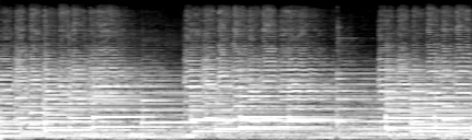
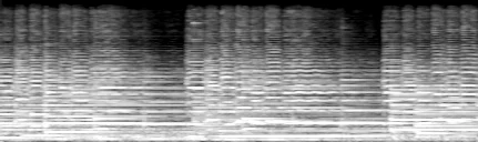
A time-frequency view of the clip — a log-mel spectrogram per channel (128 mel bins × time, low frequencies at the bottom), normalized to a grayscale image. The same make_spectrogram helper renders the reconstruction later, so the two views are directly comparable.

mel = torchaudio.transforms.MelSpectrogram(sample_rate=fs, n_fft=4096, hop_length=512)

def make_spectrogram(x_1ch):
    S = mel(x_1ch).log()
    S = ((S - S.mean()) / (3 * S.std()) + 0.5).clamp(0, 1)
    return ToPILImage()(S.flip(0))  # low frequencies at the bottom

for ch in range(x.shape[0]):
    display(make_spectrogram(x[ch]))

Audio(x.numpy(), rate=fs, normalize=False)

Resample and stack the channels

The 24 kHz checkpoint is mono, but the stereo reference is sacred — we never downmix. Instead, each channel is resampled to the model rate and the two channels are stacked as a batch of 2 with shape (2, 1, L), encoded independently in one forward pass. Bits are summed across the two channels, and the reconstruction is resampled back to 44.1 kHz before any comparison. This is the mono-on-stereo convention used by the RD harness.

x_model = taf.resample(x, fs, model_rate).unsqueeze(1).to(device)
print(f"x_model.shape = {tuple(x_model.shape)}  (batch=2 channels, mono, {model_rate} Hz)")

x_model.shape = (2, 1, 120000)  (batch=2 channels, mono, 24000 Hz)

Encode

bandwidth=6.0 selects 6 kbps per mono channel (12 kbps total for the stereo pair). The RD harness sweeps 1.5 3 6 12 24; here we stay at one operating point. The bandwidth knob works by truncating the RVQ stack: at 6 kbps the encoder keeps 8 codebooks, so each 320-sample frame becomes 8 integers in [0, 1024) — the first codebook coarsely quantizes the latent frame, and each of the 7 below it quantizes the residual of the stage above.

with torch.inference_mode():
    out = model.encode(x_model, bandwidth=6.0)
codes, scales = out.audio_codes, out.audio_scales

print(f"codes.shape = {tuple(codes.shape)}  (n_chunks, batch, n_codebooks, n_frames)")
print(f"code range  = [{codes.min().item()}, {codes.max().item()}]  of [0, {model.config.codebook_size})")
print(f"scales      = {scales}")

codes.shape = (1, 2, 8, 375)  (n_chunks, batch, n_codebooks, n_frames)
code range  = [0, 1023]  of [0, 1024)
scales      = [None]

audio_scales is [None] for this checkpoint — encodec_24khz does not normalize chunks. The 48 kHz stereo variant would carry one fp16 scale factor per chunk, which the rate accounting must include (the harness adds 16 bits per scale element when present).

Code grid

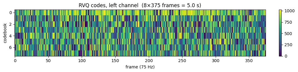
The code tensor is the audio analog of the VQ index map in the Kandinsky notebook: a small integer grid, here codebooks × frames at 75 frames/s. The raw indices carry no visible structure across rows — each codebook has its own arbitrary ordering — but this grid is the entire compressed representation.

frame_rate = model_rate / stride
plt.figure(figsize=(10, 2.5))
plt.imshow(codes[0, 0].cpu().numpy(), cmap="viridis",
           aspect="auto", interpolation="nearest")
plt.colorbar(fraction=0.025)
plt.xlabel("frame (75 Hz)")
plt.ylabel("codebook")
plt.title(f"RVQ codes, left channel  ({codes.shape[2]}×{codes.shape[3]} frames = {codes.shape[3] / frame_rate:.1f} s)")
plt.tight_layout()
plt.show()

Pack codes to bytes

Each code is 10 bits (log₂ 1024), stored here as uint16 — a generous upper bound at 16/10 = 1.6× the entropy ceiling. A real container would bit-pack at 10 bits per code or entropy-code below that; the analytic rate is what the RD harness reports.

codes_shape = tuple(codes.shape)                       # side info
buff = io.BytesIO(codes.cpu().numpy().astype(np.uint16).tobytes())

bits_per_code = int(math.log2(model.config.codebook_size))
bits_analytic = bits_per_code * codes.numel()          # both channels
bits_packed = 8 * len(buff.getbuffer())
pcm_bits = 16 * 2 * n_samples

print(f"analytic : {bits_analytic} bits = {bits_analytic / duration / 1000:.2f} kbps   CR = {pcm_bits / bits_analytic:.1f}×")
print(f"packed   : {bits_packed} bits = {bits_packed / duration / 1000:.2f} kbps   ({bits_packed / bits_analytic:.2f}× analytic)")

analytic : 60000 bits = 12.00 kbps   CR = 117.6×
packed   : 96000 bits = 19.20 kbps   (1.60× analytic)

Decode from the buffer

The decode path below reads only from buff — never from the in-memory codes tensor. The recorded codes_shape is the only other side info; a real container would carry it in a few header bytes. Decode runs the RVQ codebook lookups and the convolutional decoder at 24 kHz, then we resample back to 44.1 kHz and trim to the original length (the decoder pads to whole frames, and resampling compounds the length mismatch).

codes_rec = torch.from_numpy(
    np.frombuffer(buff.getvalue(), dtype=np.uint16).copy()
).long().reshape(codes_shape).to(device)
print(f"codes round-trip exact: {torch.equal(codes_rec, codes)}")

with torch.inference_mode():
    audio = model.decode(codes_rec, scales)[0]

x_hat = align_length(taf.resample(audio.squeeze(1).float().cpu(), model_rate, fs), n_samples)
print(f"x_hat.shape = {tuple(x_hat.shape)}")
print(f"PSNR = {psnr_db(x, x_hat):.2f} dB")

codes round-trip exact: True

x_hat.shape = (2, 220500)
PSNR = 33.59 dB

Waveform PSNR undersells neural codecs: EnCodec is trained against perceptual and adversarial losses, not MSE, so at 6 kbps per channel music is audibly artifact-y while remaining recognizable — the playable reconstruction below makes the point better than the number. (PSNR here uses the audio harness convention: −10·log₁₀(MSE) + 6.02 on the [−0.5, 0.5] signals.)

Spectrograms

The same mel view as the input, channel 0, original vs reconstruction. The model operates at 24 kHz, so everything above 12 kHz is gone from the reconstruction — but because the mel axis compresses the top octaves, the missing 12–22 kHz band shows up as a thin empty strip along the top of the image rather than the upper half it would occupy on a linear frequency axis. Below the band limit the harmonic structure is preserved, though the fine texture is visibly smoothed.

print("Original (channel 0)")
display(make_spectrogram(x[0]))
print("Reconstruction (channel 0)")
display(make_spectrogram(x_hat[0].float().cpu()))

Original (channel 0)

Reconstruction (channel 0)

Audio(x_hat.numpy(), rate=fs, normalize=False)