MP3 and Opus

Two conventional audio codecs, run through torchcodec’s in-memory AudioEncoder / AudioDecoder (backed by its bundled FFmpeg):

• MP3 (MPEG-1 Layer III, 1993) — subband filterbank + MDCT, psychoacoustic bit allocation, Huffman coding.

• Opus (RFC 6716, 2012) — the IETF standard combining the CELT transform codec with the SILK speech codec.

Unlike the learned codecs in this collection, the encoded buffer here is a real, standards-compliant byte stream — an MPEG bitstream / an Ogg-Opus container — that any player can decode. This notebook encodes a short music clip from danjacobellis/music to each format at a 64 kbps target and walks the encode → buffer → decode round trip.

import io
import torch
import torchaudio
import matplotlib.pyplot as plt
from torchvision.transforms import ToPILImage
from IPython.display import Audio
from datasets import load_dataset
from torchcodec.decoders import AudioDecoder
from torchcodec.encoders import AudioEncoder
from compressors.audio_eval import normalize_audio, align_length, psnr_db

torch.set_num_threads(8)

CLIP_INDEX = 16        # which of the 24 example files
START_SECONDS = 150.0  # offset into the file, rounded to the nearest sample
DURATION_SECONDS = 5.0 # excerpt length in seconds

Load an example clip

A 5 s stereo 44.1 kHz excerpt from one of the 24 files in the danjacobellis/music dataset (train split; each row’s audio is a torchcodec AudioDecoder). The source files are themselves MP3-encoded (this one at 320 kbps), so the “original” here is a decoded MP3 — fine for a tutorial. normalize_audio produces the zero-mean float waveform in \([-0.5, 0.5]\) that is encoded directly — no int16 round trip on the encode side.

ds = load_dataset('danjacobellis/music', split='train')
samples = ds[CLIP_INDEX]['audio'].get_all_samples()
fs = samples.sample_rate
i0 = round(START_SECONDS * fs)
x = samples.data[:, i0 : i0 + round(DURATION_SECONDS * fs)]
x = normalize_audio(x)
C, n_samples = x.shape
print(f'shape    = {tuple(x.shape)}')
print(f'duration = {n_samples / fs:.1f} s')
print(f'range    = [{x.min():.3f}, {x.max():.3f}]')

shape    = (2, 220500)
duration = 5.0 s
range    = [-0.500, 0.477]

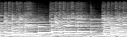
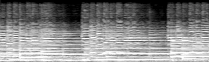
A time-frequency view of the clip — a log-mel spectrogram per channel (128 mel bins × time, low frequencies at the bottom), normalized to a grayscale image. This shows the signal the way the codecs see it: energy concentrated in time-frequency, most of it well below the Nyquist limit.

mel = torchaudio.transforms.MelSpectrogram(sample_rate=fs, n_fft=4096, hop_length=512)

def make_spectrogram(x_1ch):
    S = mel(x_1ch).log()
    S = ((S - S.mean()) / (3 * S.std()) + 0.5).clamp(0, 1)
    return ToPILImage()(S.flip(0))  # low frequencies at the bottom

for ch in range(C):
    display(make_spectrogram(x[ch]))

Audio(x.numpy(), rate=fs, normalize=False)

Encode to Opus

AudioEncoder takes the float waveform; to_tensor runs the encoder and returns the file bytes as a uint8 tensor, which we wrap in io.BytesIO. The Opus encoder accepts only 48 kHz, so sample_rate=48000 resamples internally on encode; the decoder will resample back. The requested bit_rate is a target — both encoders are VBR-ish, so the measured rate is 8 * len(buff) over the duration. The first bytes are the OggS capture pattern of an Ogg container page.

encoder = AudioEncoder(x, sample_rate=fs)
blob = encoder.to_tensor(format='opus', bit_rate=64_000, sample_rate=48_000)
buff_opus = io.BytesIO(blob.numpy().tobytes())

kbps = 8 * len(buff_opus.getbuffer()) / 1000 / (n_samples / fs)
CR = 16 * 2 * n_samples / (8 * len(buff_opus.getbuffer()))
print(f'len(buff)     = {len(buff_opus.getbuffer())} bytes')
print(f'measured rate = {kbps:.1f} kbps  (requested 64)')
print(f'CR            = {CR:.1f}x  (vs int16 stereo PCM)')
print(f'magic bytes   = {bytes(blob[:8].numpy())}')

len(buff)     = 48461 bytes
measured rate = 77.5 kbps  (requested 64)
CR            = 18.2x  (vs int16 stereo PCM)
magic bytes   = b'OggS\x00\x02\x00\x00'

Encode to MP3

Same call without the resample — MP3 codes 44.1 kHz natively. The blob starts with an ID3 metadata tag (frame sync bytes 0xFFFB... follow it).

blob = encoder.to_tensor(format='mp3', bit_rate=64_000)
buff_mp3 = io.BytesIO(blob.numpy().tobytes())

kbps = 8 * len(buff_mp3.getbuffer()) / 1000 / (n_samples / fs)
CR = 16 * 2 * n_samples / (8 * len(buff_mp3.getbuffer()))
print(f'len(buff)     = {len(buff_mp3.getbuffer())} bytes')
print(f'measured rate = {kbps:.1f} kbps  (requested 64)')
print(f'CR            = {CR:.1f}x  (vs int16 stereo PCM)')
print(f'magic bytes   = {bytes(blob[:8].numpy())}')

len(buff)     = 40586 bytes
measured rate = 64.9 kbps  (requested 64)
CR            = 21.7x  (vs int16 stereo PCM)
magic bytes   = b'ID3\x04\x00\x00\x00\x00'

Decode from the buffers

Each buffer holds a complete, playable file — write it to disk and any media player opens it; nothing project-specific is needed. Decoding reads only the bytes in the buffer, never any intermediate from the encode side. AudioDecoder(..., sample_rate=44100) resamples the Opus stream from its native 48 kHz back to 44.1 kHz; both channels pass through identical resampling, so no interchannel delay is introduced, and the resample itself is nearly transparent (a codec-free 44.1 → 48 → 44.1 round trip measures ≈ 83 dB PSNR — far above where either codec operates). The decoded clip can come back a few samples long or short (codec frame padding), so align_length trims/pads to the original length before measuring. psnr_db uses the \([0, 1]\) convention (+6.02 dB offset on the \([-0.5, 0.5]\) signals).

Expect MP3 to score a little higher in PSNR than Opus at the same rate, even where Opus sounds better. This is a property of the designs, not a fluke: MP3 quantizes MDCT coefficients directly and lowpasses what it can’t afford (zeroing high frequencies costs almost no MSE), so more bits converge toward the waveform; Opus’s CELT layer instead preserves each band’s energy (PVQ shape coding) and fills the top of its 20 kHz band with folded/synthesized content — perceptually effective, but wrong in phase, which adds waveform error. The same trade shows up in reverse below: Opus preserves the stereo image far better (SSDR).

x_hat_opus = AudioDecoder(buff_opus.getvalue(), sample_rate=fs).get_all_samples().data
x_hat_mp3 = AudioDecoder(buff_mp3.getvalue(), sample_rate=fs).get_all_samples().data
print(f'decoded shapes: opus = {tuple(x_hat_opus.shape)}, mp3 = {tuple(x_hat_mp3.shape)}')

x_hat_opus = align_length(x_hat_opus, n_samples)
x_hat_mp3 = align_length(x_hat_mp3, n_samples)
print(f'Opus PSNR = {psnr_db(x, x_hat_opus):.2f} dB')
print(f'MP3  PSNR = {psnr_db(x, x_hat_mp3):.2f} dB')

decoded shapes: opus = (2, 220500), mp3 = (2, 220500)
Opus PSNR = 44.61 dB
MP3  PSNR = 47.23 dB

Waveform detail

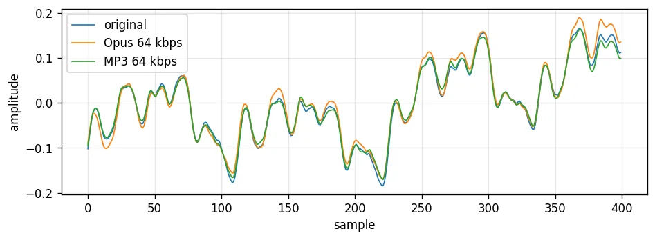
A few hundred samples of the left channel. Both reconstructions track the original closely; the error is shaped by the psychoacoustic model rather than white.

s0, n = 2 * fs, 400
plt.figure(figsize=(8, 3), dpi=120)
plt.plot(x[0, s0:s0+n], label='original', lw=1)
plt.plot(x_hat_opus[0, s0:s0+n], label='Opus 64 kbps', lw=1)
plt.plot(x_hat_mp3[0, s0:s0+n], label='MP3 64 kbps', lw=1)
plt.xlabel('sample')
plt.ylabel('amplitude')
plt.legend()
plt.grid(alpha=0.3)
plt.tight_layout()
plt.show()

Spectrograms

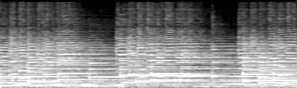
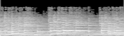
The same log-mel display as the input, now for channel 0 of the original and each reconstruction. The mel axis compresses the top octaves into the last few rows of the image, so MP3’s lowpass at this rate shows up as a thin solid-black band across the top — where the original and Opus keep visible texture — rather than the wide empty region a linear-frequency plot would show. Opus is hard to tell apart from the original at a glance. Each image is standardized to its own mean and std, so overall brightness is not comparable between panels.

for sig, title in [(x, 'original'), (x_hat_opus, 'Opus 64 kbps'), (x_hat_mp3, 'MP3 64 kbps')]:
    print(title)
    display(make_spectrogram(sig[0]))

original

Opus 64 kbps

MP3 64 kbps

Listen

The whole clip through each codec.

print('Opus 64 kbps:')
display(Audio(x_hat_opus.numpy(), rate=fs, normalize=False))
print('MP3 64 kbps:')
display(Audio(x_hat_mp3.numpy(), rate=fs, normalize=False))

Opus 64 kbps:

MP3 64 kbps:

Spatial metrics

SSDR / SRDR (Watcharasupat & Lerch, ICASSP 2024) decompose the stereo error into a spatial term (interchannel gain/delay/leakage) and a residual term — see compressors.spatial_audio_quality. MP3’s joint-stereo coding leaks more between channels (lower SSDR) while keeping a cleaner residual (higher SRDR) than Opus at this rate.

from compressors.spatial_audio_quality import ssdr_srdr

for name, x_hat in [('Opus', x_hat_opus), ('MP3', x_hat_mp3)]:
    m = ssdr_srdr(x, x_hat, fs)
    print(f"{name}: SSDR = {m['SSDR']:.2f} dB   SRDR = {m['SRDR']:.2f} dB")

Opus: SSDR = 42.00 dB   SRDR = 17.79 dB

MP3: SSDR = 25.41 dB   SRDR = 21.57 dB