LiVeAction (stereo audio)

@inproceedings{jacobellis2026liveaction,
  title={{LiVeAction}: Lightweight, Versatile, and Asymmetric Codec Design for Real-time Operation},
  author={Jacobellis, Dan and Yadwadkar, Neeraja J.},
  booktitle={IEEE Data Compression Conference (DCC)},
  year={2026},
  note={in press},
  url={https://ut-sysml.github.io/liveaction}
}

Project webpage

Github

Pre-trained model weights

The same codec family covers images, audio, video, and more. This notebook walks the stereo audio checkpoint (musdb_stereo_f512c16) through a full encode → buffer → decode round trip on a five-second music excerpt; the image sibling is LiVeAction.

import io, math, torch, torchaudio, matplotlib.pyplot as plt
import PIL.Image
from IPython.display import Audio
from datasets import load_dataset
from torchvision.transforms import ToPILImage

from compressors.audio_eval import normalize_audio, pad_audio, psnr_db
from compressors.liveaction_audio._codec import (
    load_codec,
    encode_to_latent,
    latent_to_tiff_bytes,
    decode_from_tiff_bytes,
)

device = 'cuda' if torch.cuda.is_available() else 'cpu'
dtype = torch.bfloat16  # the canonical inference dtype for this checkpoint
print(f'device={device}  dtype={dtype}')

device=cuda  dtype=torch.bfloat16

Load the codec

A single native operating point: F=512 sets the wavelet packet depth J = log2(F) = 9, and 16 latent channels give a 64× dimensionality reduction of the stereo waveform. The weights live in the pre-rename danjacobellis/autocodec repository.

model, config = load_codec(device=device, torch_dtype=dtype)
J = int(math.log2(config.F))
DR = config.input_channels * config.F // config.latent_dim
print(f'F          = {config.F}')
print(f'J          = {J}')
print(f'latent_dim = {config.latent_dim}')
print(f'channels   = {config.input_channels}')
print(f'DR         = {DR}')

F          = 512
J          = 9
latent_dim = 16
channels   = 2
DR         = 64

Load an example clip

The danjacobellis/music dataset holds 24 example songs (the source files are themselves MP3 at ~258 kbps); each row’s audio field decodes via torchcodec. We take a five-second stereo excerpt at 44.1 kHz, normalize to a zero-mean signal in \([-0.5, 0.5]\), and pad to a multiple of \(2^{16}\) — the same convention as the rate–distortion harness.

CLIP_INDEX = 16        # which of the 24 example files
START_SECONDS = 150.0  # offset into the file, rounded to the nearest sample
DURATION_SECONDS = 5.0 # excerpt length in seconds

ds = load_dataset("danjacobellis/music", split="train")
samples = ds[CLIP_INDEX]["audio"].get_all_samples()
fs = samples.sample_rate
i0 = round(START_SECONDS * fs)
x = samples.data[:, i0 : i0 + round(DURATION_SECONDS * fs)]
x = normalize_audio(x)
n_samples = x.shape[-1]
x_in = pad_audio(x.unsqueeze(0), 2**16).to(device).to(dtype)
print(f'fs:     {fs} Hz')
print(f'clip:   {tuple(x.shape)} {x.dtype}')
print(f'padded: {tuple(x_in.shape)} {x_in.dtype}')

fs:     44100 Hz
clip:   (2, 220500) torch.float32
padded: (1, 2, 262144) torch.bfloat16

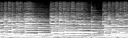
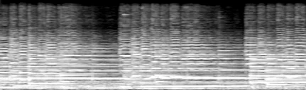
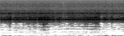
We visualize the clip as a log-mel spectrogram per channel, rendered directly as a PIL image with low frequencies at the bottom. The same make_spectrogram helper is reused to visualize the reconstruction at the end.

mel = torchaudio.transforms.MelSpectrogram(sample_rate=fs, n_fft=4096, hop_length=512)

def make_spectrogram(x_1ch):
    S = mel(x_1ch).log()
    S = ((S - S.mean()) / (3 * S.std()) + 0.5).clamp(0, 1)
    return ToPILImage()(S.flip(0))  # low frequencies at the bottom

for ch, name in enumerate(['left', 'right']):
    print(f'{name} channel')
    display(make_spectrogram(x[ch]))

Audio(x.numpy(), rate=fs)

left channel

right channel

Analysis transform

A depth-9 wavelet packet transform followed by a lightweight learned encoder maps the stereo waveform to 16 latent channels at 1/512 the sample rate.

with torch.no_grad():
    z = model.encode(x_in)
print(f'continuous latent shape: {tuple(z.shape)}')
print(f'{x_in.numel()} padded samples in, {z.numel()} latent values out: {x_in.numel() // z.numel()}x dimensionality reduction')

continuous latent shape: (1, 16, 512)
524288 padded samples in, 8192 latent values out: 64x dimensionality reduction

Companding

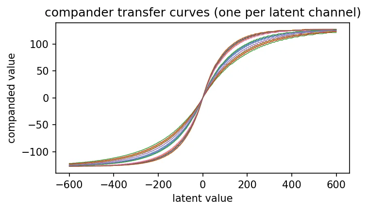
Before quantization, each latent channel passes through a learned Laplace CDF scaled to \([-127, 127]\). The nonlinearity allocates the 8-bit integer grid according to a Laplace prior on the latents, so a plain round() behaves like a non-uniform quantizer. (encode_to_latent bundles companding and rounding; we expand them here so each stage is visible.)

ramp = torch.linspace(-600, 600, 2401, device=device, dtype=dtype)
with torch.no_grad():
    curves = model.quantize.compand(ramp.view(1, 1, -1).expand(1, config.latent_dim, -1))

plt.figure(figsize=(5, 3), dpi=150)
plt.plot(ramp.float().cpu(), curves[0].float().cpu().T, linewidth=0.7)
plt.xlabel('latent value')
plt.ylabel('companded value')
plt.title('compander transfer curves (one per latent channel)')
plt.tight_layout()
plt.show()

with torch.no_grad():
    z_c = model.quantize.compand(z)
print(f'companded latent range: [{z_c.min().item():.1f}, {z_c.max().item():.1f}]  (grid spans [-127, 127])')

companded latent range: [-8.0, 12.0]  (grid spans [-127, 127])

Rounding

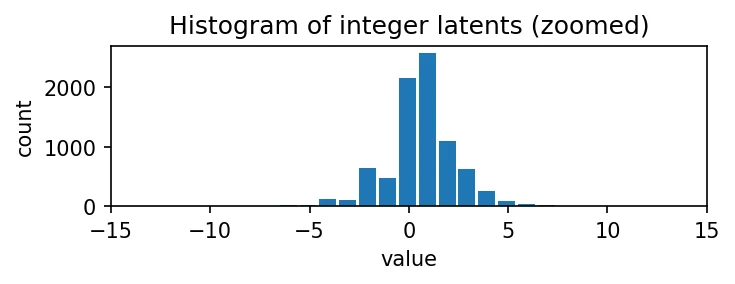
Rounding the companded latent to integers is the lossy step.

latent = z_c.round()
err = (z_c - latent).float()
qsnr = 10 * (z_c.float().pow(2).mean() / err.pow(2).mean()).log10().item()
print(f'integer latent range:    [{int(latent.min())}, {int(latent.max())}]')
print(f'latent quantization SNR: {qsnr:.2f} dB')

plt.figure(figsize=(5, 2), dpi=150)
plt.hist(latent.float().cpu().flatten(), range=(-127.5, 127.5), bins=255, width=0.85)
plt.xlim([-15, 15])
plt.title('Histogram of integer latents (zoomed)')
plt.xlabel('value')
plt.ylabel('count')
plt.tight_layout()
plt.show()

integer latent range:    [-8, 12]
latent quantization SNR: 19.78 dB

Latent as a CMYK image (entropy coding)

The integer latent is folded to 2-D, packed four channels at a time into the planes of an 8-bit CMYK image, and saved as a TIFF with tiff_adobe_deflate compression. Deflate inside a TIFF container is the entropy coder; the CMYK packing is just a 4-channel carrier. The encoder’s entire output is a single buffer of TIFF bytes.

blob = latent_to_tiff_bytes(latent.cpu(), config.latent_dim)
buff = io.BytesIO(blob)

img = PIL.Image.open(io.BytesIO(buff.getvalue()))
img.load()
print(f'packed image: {img.size} {img.mode}')
display(img.convert('RGB').resize((8 * img.width, 8 * img.height), resample=PIL.Image.Resampling.NEAREST))

packed image: (32, 64) CMYK

Dimensionality reduction is not bit rate. The autoencoder reduces values by 64× (DR), but each latent is stored at 8 bits versus the PCM’s 16, so even raw packing would give CR = 128 — and deflate pushes well past that because the companded latents concentrate on a few small integers. The gap between DR and CR is the whole reason the entropy coding stage exists. One caveat at this clip length: padding to a multiple of \(2^{16}\) stretches 220,500 samples to 262,144 (~19% overhead), so the measured CR — denominated in the original samples — falls ~19% short of the \(\mathrm{DR} \cdot 16 / \text{bits per latent value}\) identity, which is exact in padded samples.

n_bytes = len(buff.getbuffer())
kbps = 8 * n_bytes / (n_samples / fs) / 1000
CR = 16 * 2 * n_samples / (8 * n_bytes)
bits_per_latent_value = 8 * n_bytes / latent.numel()
print(f'compressed size:       {n_bytes} bytes')
print(f'bitrate:               {kbps:.2f} kbps')
print(f'bits per latent value: {bits_per_latent_value:.3f}')
print(f'compression ratio:     {CR:.1f}  (vs DR = {DR})')
print(f'DR * 16 / bits_per_latent_value = {DR * 16 / bits_per_latent_value:.1f}')

compressed size:       3332 bytes
bitrate:               5.33 kbps
bits per latent value: 3.254
compression ratio:     264.7  (vs DR = 64)
DR * 16 / bits_per_latent_value = 314.7

Decode from the buffer

The decoder reads only the TIFF bytes in buff (plus the clip length as side info) — the in-memory latent is never reused. decode_from_tiff_bytes reopens the image, unfolds the latent, runs the learned decoder, and clamps.

with torch.no_grad():
    x_hat = decode_from_tiff_bytes(model, buff.getvalue(), config.latent_dim, n_samples, device, dtype)
x_hat = x_hat.float().cpu()

print(f'kbps = {kbps:.2f}')
print(f'PSNR = {psnr_db(x, x_hat):.2f} dB')

kbps = 5.33
PSNR = 32.66 dB

Reconstruction

The same make_spectrogram view of channel 0, before and after the round trip. The harmonic stack in the bass and low mids comes through nearly intact; higher up, the fine harmonic lines blur together and the quiet gaps between phrases in the top octaves partially fill in — the visible cost of the 64× reduction at this single operating point.

print('original (channel 0)')
display(make_spectrogram(x[0]))
print('reconstruction (channel 0)')
display(make_spectrogram(x_hat[0]))

Audio(x_hat.numpy(), rate=fs)

original (channel 0)

reconstruction (channel 0)

This codec codes the two channels jointly, so the spatial metrics SSDR/SRDR (Watcharasupat & Lerch, ICASSP 2024) are meaningful: cross-channel leakage shows up as spatial distortion.

from compressors.spatial_audio_quality import ssdr_srdr
metrics = ssdr_srdr(x, x_hat, fs)
print(f"SSDR = {metrics['SSDR']:.2f} dB")
print(f"SRDR = {metrics['SRDR']:.2f} dB")

SSDR = 11.15 dB
SRDR = 4.99 dB