Mimi

@article{defossez2024moshi,
  title={Moshi: a speech-text foundation model for real-time dialogue},
  author={D{\'e}fossez, Alexandre and Mazar{\'e}, Laurent and Orsini, Manu and Royer, Am{\'e}lie and P{\'e}rez, Patrick and J{\'e}gou, Herv{\'e} and Grave, Edouard and Zeghidour, Neil},
  journal={arXiv preprint arXiv:2410.00037},
  year={2024}
}

arXiv

Pre-trained model weights

Mimi is the neural audio codec inside Moshi, Kyutai’s real-time speech-text foundation model. It is a 24 kHz mono RVQ codec with a split quantizer: the first codebook is semantic — distilled from WavLM representations so a language model can consume it directly — and the remaining codebooks are acoustic. This notebook walks the encode → buffer → decode round trip on a 5 s music excerpt at num_quantizers=8.

import io
import math
import numpy as np
import torch
import torchaudio
import torchaudio.functional as taf
import matplotlib.pyplot as plt
from datasets import load_dataset
from torchvision.transforms import ToPILImage
from IPython.display import Audio

from compressors.audio_eval import normalize_audio, align_length, psnr_db
from compressors.mimi.evaluate_rate_distortion import load_model

Load the codec

device = "cuda:1" if torch.cuda.is_available() else "cpu"
torch.set_num_threads(8)

model = load_model(device, torch.float32)
cfg = model.config
bits_per_code = int(math.log2(cfg.codebook_size))

print(f"sampling rate       = {cfg.sampling_rate} Hz (mono)")
print(f"codebook size       = {cfg.codebook_size}  ({bits_per_code} bits/code)")
print(f"frame rate          = {cfg.frame_rate} Hz")
print(f"max quantizers      = {cfg.num_quantizers}")
print(f"semantic quantizers = {cfg.num_semantic_quantizers}")

Skipping import of cpp extensions due to incompatible torch version 2.11.0+cu130 for torchao version 0.15.0             Please see https://github.com/pytorch/ao/issues/2919 for more info

sampling rate       = 24000 Hz (mono)
codebook size       = 2048  (11 bits/code)
frame rate          = 12.5 Hz
max quantizers      = 32
semantic quantizers = 1

Load an example clip

The clip is an excerpt from danjacobellis/music (24 example files, train split); each row’s audio is a torchcodec AudioDecoder, and the source files are themselves MP3 at ~258 kbps. The parameters below pick one file and a 5 s stereo excerpt at 44.1 kHz. Normalization follows the audio harness convention: cast to float, subtract the mean, divide by the peak, divide by 2 → \([-0.5, 0.5]\).

CLIP_INDEX = 16        # which of the 24 example files
START_SECONDS = 150.0  # offset into the file, rounded to the nearest sample
DURATION_SECONDS = 5.0 # excerpt length in seconds

ds = load_dataset("danjacobellis/music", split="train")
samples = ds[CLIP_INDEX]["audio"].get_all_samples()
fs = samples.sample_rate
i0 = round(START_SECONDS * fs)
x = samples.data[:, i0 : i0 + round(DURATION_SECONDS * fs)]
x = normalize_audio(x)
n_samples = x.shape[-1]
duration = n_samples / fs
print(f"x.shape = {tuple(x.shape)}  fs = {fs} Hz  range = [{x.min().item():.3f}, {x.max().item():.3f}]  ({duration:.1f} s)")

x.shape = (2, 220500)  fs = 44100 Hz  range = [-0.500, 0.477]  (5.0 s)

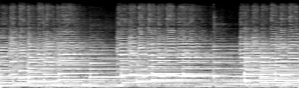
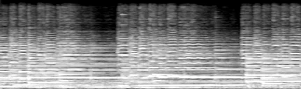
A log-mel spectrogram of each channel, rendered as a PIL image with low frequencies at the bottom. The same make_spectrogram helper is reused later to compare the reconstructions against the original.

mel = torchaudio.transforms.MelSpectrogram(sample_rate=fs, n_fft=4096, hop_length=512)

def make_spectrogram(x_1ch):
    S = mel(x_1ch).log()
    S = ((S - S.mean()) / (3 * S.std()) + 0.5).clamp(0, 1)
    return ToPILImage()(S.flip(0))  # low frequencies at the bottom

for ch in range(2):
    display(make_spectrogram(x[ch]))

Audio(np.clip(x.numpy(), -1, 1), rate=fs, normalize=False)

Resample and stack

Mimi is a mono model. We never downmix: the stereo signal is resampled 44.1 kHz → 24 kHz and the two channels are stacked as a batch of 2 with shape (2, 1, L), encoded independently, and the bits summed.

model_rate = cfg.sampling_rate
x_model = taf.resample(x, fs, model_rate)
x_in = x_model.unsqueeze(1).to(device)
print(f"x_in.shape = {tuple(x_in.shape)}  at {model_rate} Hz")

x_in.shape = (2, 1, 120000)  at 24000 Hz

Encode

We encode at num_quantizers=8 of the 32 available; the RD harness sweeps 1 2 4 8 16 32. At 12.5 Hz, the 5 s excerpt becomes just ~63 frames per channel — EnCodec runs at 75 Hz, so Mimi produces 6× fewer positions for the same audio, which is what makes it cheap to interleave into an LM token stream.

with torch.inference_mode():
    codes = model.encode(x_in, num_quantizers=8).audio_codes

n_frames = codes.shape[-1]
print(f"codes.shape = {tuple(codes.shape)}  dtype = {codes.dtype}")
print(f"code values ∈ [{int(codes.min())}, {int(codes.max())}]  of [0, {cfg.codebook_size})")
print(f"frame rate  = {n_frames / (x_model.shape[-1] / model_rate):.2f} Hz")

codes.shape = (2, 8, 63)  dtype = torch.int64
code values ∈ [0, 2043]  of [0, 2048)
frame rate  = 12.60 Hz

Code grid

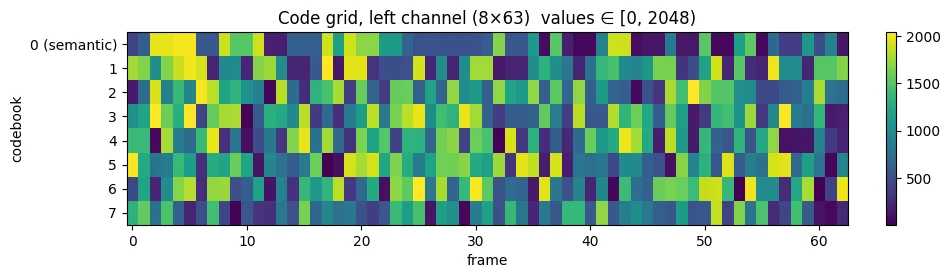
The (num_quantizers, n_frames) grid for the left channel. Row 0 is the semantic codebook — it carries what is in the signal; rows 1–7 are acoustic refinements.

plt.figure(figsize=(10, 2.5))
plt.imshow(codes[0].cpu().numpy(), aspect="auto", cmap="viridis", interpolation="nearest")
plt.colorbar(fraction=0.02)
plt.yticks(range(8), ["0 (semantic)"] + [str(i) for i in range(1, 8)])
plt.xlabel("frame")
plt.ylabel("codebook")
plt.title(f"Code grid, left channel ({codes.shape[1]}×{n_frames})  values ∈ [0, {cfg.codebook_size})")
plt.show()

Semantic-only decode

As an aside: encoding with num_quantizers=1 keeps only the semantic codebook. The decode preserves what is happening — rhythm, broad timbre — while discarding nearly all acoustic detail.

with torch.inference_mode():
    codes_sem = model.encode(x_in, num_quantizers=1).audio_codes
    y_sem = model.decode(codes_sem).audio_values.squeeze(1)
x_hat_sem = align_length(taf.resample(y_sem.float().cpu(), model_rate, fs), n_samples)
print(f"semantic-only: codes.shape = {tuple(codes_sem.shape)}  PSNR = {psnr_db(x, x_hat_sem):.2f} dB")
Audio(np.clip(x_hat_sem.numpy(), -1, 1), rate=fs, normalize=False)

semantic-only: codes.shape = (2, 1, 63)  PSNR = 25.80 dB

Pack codes to bytes

The compressed representation is the integer code grid. We record its shape as side info and pack the codes as uint16 into a BytesIO buffer — everything the decoder reads comes from this buffer.

codes_np = codes.cpu().numpy().astype(np.uint16)
codes_shape = codes_np.shape
buff = io.BytesIO(codes_np.tobytes())
n_bytes = len(buff.getbuffer())
print(f"side info: codes_shape = {codes_shape}")
print(f"packed uint16 bytes = {n_bytes}")

side info: codes_shape = (2, 8, 63)
packed uint16 bytes = 2016

total_bits = bits_per_code * codes.numel()   # summed over both channels
kbps = total_bits / duration / 1000
cr = 16 * 2 * n_samples / total_bits
kbps_packed = 8 * n_bytes / duration / 1000

print(f"analytic : {total_bits} bits = {kbps:.2f} kbps   CR = {cr:.0f}× vs int16 stereo PCM")
print(f"packed   : {8 * n_bytes} bits = {kbps_packed:.2f} kbps")

analytic : 11088 bits = 2.22 kbps   CR = 636× vs int16 stereo PCM
packed   : 16128 bits = 3.23 kbps

The analytic rate charges \(\log_2(2048) = 11\) bits per code. The packed buffer stores each code in 16 bits, a 45% overhead; a real container would bit-pack to 11 bits or entropy-code the indices, so the analytic number is the honest rate and the buffer is just a convenient transport.

Decode from the buffer

The decode below reads only from buff (plus the recorded shape): parse the uint16 codes, look them up through the decoder, and resample back to 44.1 kHz stereo.

codes_rec = np.frombuffer(buff.getvalue(), dtype=np.uint16).reshape(codes_shape)
print(f"bit-exact code round trip: {np.array_equal(codes_rec, codes.cpu().numpy())}")

with torch.inference_mode():
    y = model.decode(torch.from_numpy(codes_rec.astype(np.int64)).to(device)).audio_values
y = y.squeeze(1)                                      # (2, 1, L) → (2, L)
x_hat = taf.resample(y.float().cpu(), model_rate, fs)
x_hat = align_length(x_hat, n_samples)
print(f"x_hat.shape = {tuple(x_hat.shape)}")

bit-exact code round trip: True
x_hat.shape = (2, 220500)

Reconstruction quality

Mimi is a speech codec being run on stereo music, far outside its training distribution — expect heavy artifacts, and treat the waveform PSNR below (the harnesses’ \([-0.5, 0.5]\) convention) as a rate-matched comparison point, not a recommendation. That comparison is exactly why it is in the registry.

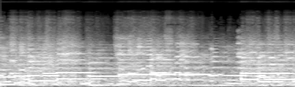
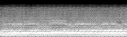
The mel spectrograms below tell the story. The original is dense with parallel harmonic lines, and energy reaches the top of the band in bursts at the loud onsets, with dark gaps in the highs between phrases. The n_q=8 reconstruction preserves the envelope and the low-frequency energy, but the harmonic lines smear into a broadband wash and the top of the band is visibly attenuated. The semantic-only (n_q=1) reconstruction goes much further: the harmonic structure is essentially gone, leaving a diffuse texture in which little more than the overall envelope survives.

print(f"PSNR = {psnr_db(x, x_hat):.2f} dB    {kbps:.2f} kbps (analytic)    CR = {cr:.0f}×")

PSNR = 29.15 dB    2.22 kbps (analytic)    CR = 636×

for label, sig in [("Original", x),
                   ("Reconstruction (n_q=8)", x_hat),
                   ("Semantic-only (n_q=1)", x_hat_sem)]:
    print(label)
    display(make_spectrogram(sig[0].float().cpu()))

Original

Reconstruction (n_q=8)

Semantic-only (n_q=1)

Audio(np.clip(x_hat.numpy(), -1, 1), rate=fs, normalize=False)