FRAPPE v2 — stereo audio

@inproceedings{jacobellis2026frappe,
  title={FRAPPE: Full Input, Residual Output Autoencoding with Projection Pursuit Encoder},
  author={Jacobellis, Dan and Yadwadkar, Neeraja J.},
  note={under review},
  year={2026},
  url={https://ut-sysml.github.io/FRAPPE}
}

Project webpage · GitHub

The differences between FRAPPE v1 and v2:

• Support for 1d and 3d signals (e.g. audio and video). This notebook is the stereo-audio instance (dim=1, 2 channels); see FRAPPE.ipynb for the v1 image tutorial.

• Training occurs in channel groups. This gives fewer operating points to choose from but makes training significantly faster.

The codec (campaign run B1) is loaded from the Hugging Face hub through the compressors.frappe_v2_audio public API — there is no local checkpoint or training code in this notebook.

import torch, numpy as np, matplotlib.pyplot as plt
import PIL.Image, PIL.ImageOps, torchaudio
from IPython.display import Audio, display
from datasets import load_dataset
from torchvision.transforms import ToPILImage
from torchvision.transforms.v2.functional import to_pil_image
from compressors.frappe_v2_audio import load_all_codecs, encode_latents, decode_latents

Load the codec

device = 'cuda:0'
config, models = load_all_codecs(device=device)          # one MergedAutoencoder per operating point

ops = list(config.cumulative_channels)                    # channel-truncation points (group boundaries)
cum = [0] + ops
group_sizes = [cum[i + 1] - cum[i] for i in range(len(ops))]
ps_groups   = [config.ps[cum[i]] for i in range(len(ops))]
max_ps      = max(config.ps)
n_trained   = max(ops)
model       = models[n_trained]                           # full-rate model (all channels)

print(f'modality      = {config.modality}  (dim={config.dim})')
print(f'channels      = {config.input_channels}')
print(f'ps per group  = {ps_groups}')
print(f'group_sizes   = {group_sizes}')
print(f'boundaries    = {ops}  (cumulative channels)')
print(f'decoder ps    = {config.decoder_ps}   decoder_dim = {config.decoder_dim}')
for s, (ps_s, start, end) in enumerate(model.scale_groups):
    print(f'  scale {s+1}: ps={ps_s:>5}  channels {start+1}-{end}  (latent rate 1/{ps_s})')

modality      = audio  (dim=1)
channels      = 2
ps per group  = [256, 256, 128, 64, 32, 16, 8]
group_sizes   = [4, 5, 6, 6, 12, 9, 9]
boundaries    = [4, 9, 15, 21, 33, 42, 51]  (cumulative channels)
decoder ps    = 128   decoder_dim = 1024
  scale 1: ps=  256  channels 1-9  (latent rate 1/256)
  scale 2: ps=  128  channels 10-15  (latent rate 1/128)
  scale 3: ps=   64  channels 16-21  (latent rate 1/64)
  scale 4: ps=   32  channels 22-33  (latent rate 1/32)
  scale 5: ps=   16  channels 34-42  (latent rate 1/16)
  scale 6: ps=    8  channels 43-51  (latent rate 1/8)

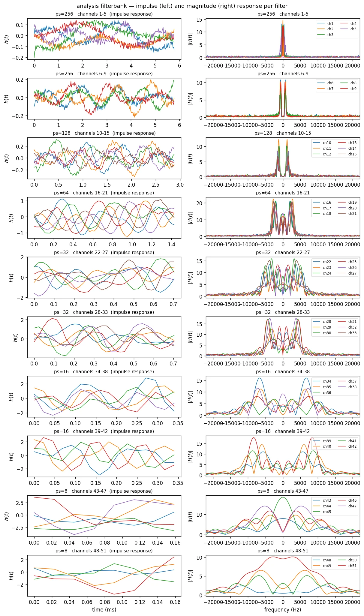
Analysis filterbank

def chunk_sizes(n, max_per=6):
    """Split n channels into as-even-as-possible panels of <= max_per (3-6 each for our groups)."""
    k = max(1, -(-n // max_per))                # ceil(n / max_per)
    return [n // k + (1 if i < n % k else 0) for i in range(k)]

N = 3001
fs_hz = 44100                                              # input sample rate (stereo 44.1 kHz)
freqs = np.fft.fftshift(np.fft.fftfreq(N)) * fs_hz         # frequency in Hz, [-22050, 22050)

# Build one panel per chunk of channels: (ps, ch_lo, ch_hi, filters)
panels = []
for s, (ps_s, start, end) in enumerate(model.scale_groups):
    W = model.encoders[s][0].weight.data.cpu().numpy().mean(1)   # (C, ps), mean over L/R input
    off = 0
    for sz in chunk_sizes(end - start):
        panels.append((ps_s, start + off + 1, start + off + sz, W[off:off + sz]))
        off += sz

# Left column: impulse response (filter taps).  Right column: magnitude response.
fig, axes = plt.subplots(len(panels), 2, figsize=(10, 1.7 * len(panels)), dpi=120,
                         constrained_layout=True)
axes = np.atleast_2d(axes)
for (ax_imp, ax_mag), (ps_s, ch_lo, ch_hi, filt) in zip(axes, panels):
    t_ms = np.arange(filt.shape[1]) / fs_hz * 1e3          # tap index -> time in ms
    for c, h in enumerate(filt, start=ch_lo):
        H = np.fft.fftshift(np.fft.fft(h, N))
        ax_imp.plot(t_ms, h, lw=1.0, label=f'ch{c}')
        ax_mag.plot(freqs, np.abs(H), lw=1.0, label=f'ch{c}')
    ax_imp.set_title(f'ps={ps_s}   channels {ch_lo}-{ch_hi}  (impulse response)', fontsize=9)
    ax_mag.set_title(f'ps={ps_s}   channels {ch_lo}-{ch_hi}', fontsize=9)
    ax_mag.set_xlim(-fs_hz / 2, fs_hz / 2)
    ax_imp.set_ylabel(r'$h(t)$')
    ax_mag.set_ylabel(r'$|H(f)|$')
    ax_mag.legend(fontsize=7, loc='upper right', framealpha=0.6, ncol=2)
axes[-1, 0].set_xlabel('time (ms)')
axes[-1, 1].set_xlabel('frequency (Hz)')
fig.suptitle('analysis filterbank — impulse (left) and magnitude (right) response per filter', fontsize=11)
plt.show()

Load an example clip

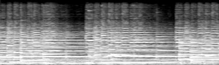
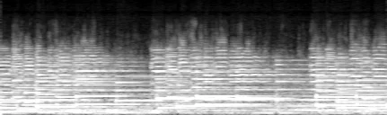
The danjacobellis/music dataset (private due to copyright) holds 24 stereo music tracks. The source files are lossy MP3 but at near-lossless rates. We use a five-second stereo 44.1 kHz excerpt, normalized to [-1, 1], cropped to a multiple of the coarsest patch size max(ps).

CLIP_INDEX = 16
START_SECONDS = 150.0
DURATION_SECONDS = 5.0

ds = load_dataset("danjacobellis/music", split="train")
samples = ds[CLIP_INDEX]["audio"].get_all_samples()
fs = samples.sample_rate
i0 = round(START_SECONDS * fs)
x = samples.data[:, i0 : i0 + round(DURATION_SECONDS * fs)]

# normalize to the codec convention: zero-mean, peak-normalized to [-1, 1]
x = x.to(torch.float)
x = x - x.mean()
x = x / (x.abs().max() + 1e-8)
L = max_ps * (x.shape[-1] // max_ps)     # crop to a multiple of max(ps)
x = x[..., :L]
n_samples = x.shape[-1]
x_in = x.unsqueeze(0).to(device)
print(f'fs       = {fs} Hz')
print(f'clip     = {tuple(x.shape)}  ({n_samples / fs:.1f} s),  range [{x.min():.2f}, {x.max():.2f}]')
print(f'model in = {tuple(x_in.shape)}  (length divisible by max(ps)={max_ps})')

fs       = 44100 Hz
clip     = (2, 220416)  (5.0 s),  range [-1.00, 0.95]
model in = (1, 2, 220416)  (length divisible by max(ps)=256)

mel = torchaudio.transforms.MelSpectrogram(sample_rate=fs, n_fft=4096, hop_length=512)

def make_spectrogram(x_1ch):
    S = mel(x_1ch).log()
    S = ((S - S.mean()) / (3 * S.std()) + 0.5).clamp(0, 1)
    return ToPILImage()(S.flip(0))  # low frequencies at the bottom

for ch, name in enumerate(['left', 'right']):
    print(f'{name} channel')
    display(make_spectrogram(x[ch]))

Audio(x.numpy(), rate=fs)

left channel

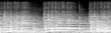
right channel

Analysis transform

with torch.no_grad():
    latents = model.encode(x_in)        # list of (1, C_scale, L_scale), companded but not yet rounded
n_latent_values = sum(z.numel() for z in latents)
print(f'{x_in.numel()} input samples -> {n_latent_values} latent values '
      f'({n_latent_values / x_in.numel():.2f}x — overcomplete)')
for s, z in enumerate(latents):
    print(f'  scale {s+1} (ps={model.scale_groups[s][0]:>5}): latent {tuple(z.shape)}  '
          f'range [{z.min():.1f}, {z.max():.1f}]')

440832 input samples -> 493353 latent values (1.12x — overcomplete)
  scale 1 (ps=  256): latent (1, 9, 861)  range [-5.7, 5.7]
  scale 2 (ps=  128): latent (1, 6, 1722)  range [-3.9, 5.2]
  scale 3 (ps=   64): latent (1, 6, 3444)  range [-11.9, 12.9]
  scale 4 (ps=   32): latent (1, 12, 6888)  range [-11.1, 11.2]
  scale 5 (ps=   16): latent (1, 9, 13776)  range [-7.7, 7.4]
  scale 6 (ps=    8): latent (1, 9, 27552)  range [-10.9, 10.2]

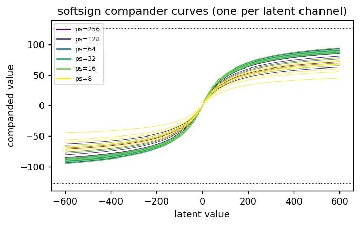
Companding

ramp = torch.linspace(-600, 600, 2401, device=device)
plt.figure(figsize=(5.5, 3.5), dpi=130)
colors = plt.cm.viridis(np.linspace(0, 1, len(model.scale_groups)))
for s, (ps_s, start, end) in enumerate(model.scale_groups):
    C = end - start
    with torch.no_grad():
        curves = model.encoders[s][1](ramp.view(1, 1, -1).expand(1, C, -1))   # softsign compander
    plt.plot(ramp.cpu(), curves[0].cpu().T, lw=0.5, color=colors[s])
    plt.plot([], [], color=colors[s], label=f'ps={ps_s}')   # legend proxy
plt.axhline(127, ls=':', c='k', lw=0.6); plt.axhline(-127, ls=':', c='k', lw=0.6)
plt.xlabel('latent value'); plt.ylabel('companded value')
plt.title('softsign compander curves (one per latent channel)')
plt.legend(fontsize=7); plt.tight_layout(); plt.show()

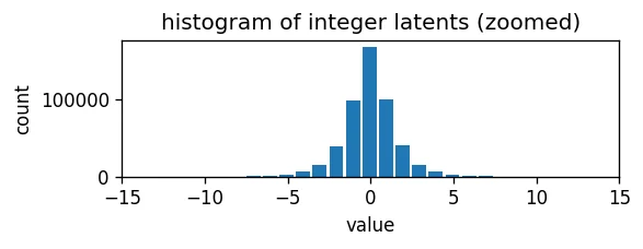
Rounding

latents_q = [z.round().clamp(-127, 127) for z in latents]
z_c = torch.cat([z.flatten() for z in latents])
z_q = torch.cat([z.flatten() for z in latents_q])
qsnr = 10 * (z_c.pow(2).mean() / (z_c - z_q).pow(2).mean()).log10().item()
print(f'integer latent range:    [{int(z_q.min())}, {int(z_q.max())}]')
print(f'latent quantization SNR: {qsnr:.2f} dB')

plt.figure(figsize=(5, 2), dpi=120)
plt.hist(z_q.cpu().numpy(), range=(-127.5, 127.5), bins=255, width=0.85)
plt.xlim([-15, 15]); plt.title('histogram of integer latents (zoomed)')
plt.xlabel('value'); plt.ylabel('count'); plt.tight_layout(); plt.show()

latents_q = [z.to(torch.int8) for z in latents_q]

integer latent range:    [-12, 13]
latent quantization SNR: 14.58 dB

Stacking latents and entropy coding using a lossless image codec

def scale_for_display(img, target=768):
    """Autocontrast, then integer-upscale (nearest) so the latent image is visible."""
    img = PIL.ImageOps.autocontrast(img)
    s = max(1, target // max(img.size))
    return img.resize((img.width * s, img.height * s), PIL.Image.NEAREST)

# encode_latents (from compressors.frappe_v2_audio) packs each per-scale int8 latent
# (1, C, L) into a (C, L) grayscale JPEG-LS stream, length-prefixed so the blob is
# self-describing. Per-scale payload sizes are recovered by encoding each scale alone.
blob = encode_latents(latents_q)
sizes = [len(encode_latents([z])) - 4 for z in latents_q]   # JPEG-LS payload bytes per scale (minus 4-byte prefix)

WIN = 256   # display only the first WIN time steps of each scale (the codec sees the full length)
for s, (z, sz) in enumerate(zip(latents_q, sizes)):
    print(f'scale {s+1} (ps={model.scale_groups[s][0]:>5}, {z.shape[1]:>2}ch x {z.shape[2]}):  {sz:>8,} bytes')
    img = to_pil_image((z[0, :, :WIN].cpu().long() + 127).to(torch.uint8))
    display(scale_for_display(img))

scale 1 (ps=  256,  9ch x 861):     2,788 bytes

scale 2 (ps=  128,  6ch x 1722):     3,186 bytes

scale 3 (ps=   64,  6ch x 3444):     9,344 bytes

scale 4 (ps=   32, 12ch x 6888):    35,323 bytes

scale 5 (ps=   16,  9ch x 13776):    30,802 bytes

scale 6 (ps=    8,  9ch x 27552):    68,236 bytes

n_bits = len(blob) * 8
kbps = n_bits / (n_samples / fs) / 1000
CR = 16 * config.input_channels * n_samples / n_bits
bits_per_latent_value = n_bits / n_latent_values
print(f'compressed size:       {len(blob):,} bytes')
print(f'bitrate:               {kbps:.2f} kbps')
print(f'bits per latent value: {bits_per_latent_value:.3f}')
print(f'compression ratio:     {CR:.1f}x  (vs 16-bit stereo PCM,  {n_trained} ch)')

compressed size:       149,703 bytes
bitrate:               239.62 kbps
bits per latent value: 2.428
compression ratio:     5.9x  (vs 16-bit stereo PCM,  51 ch)

Decode latents

latents_dec = decode_latents(blob, model.scale_groups)
assert all(torch.equal(a.cpu(), b.cpu()) for a, b in zip(latents_dec, latents_q)), 'entropy round-trip mismatch'
print('entropy round-trip: latents recovered exactly from the byte blob ✓')

with torch.no_grad():
    x_hat = model.decode([z.to(device) for z in latents_dec]).clamp(-1, 1)
x_hat = x_hat[0].float().cpu()

# PSNR on the [0,1]-mapped signal (FRAPPE convention: x/2 + 0.5, no offset)
psnr = -10 * torch.nn.functional.mse_loss(x / 2 + 0.5, x_hat / 2 + 0.5).log10().item()
print(f'kbps = {kbps:.2f}')
print(f'PSNR = {psnr:.2f} dB   ({n_trained} ch)')

entropy round-trip: latents recovered exactly from the byte blob ✓
kbps = 239.62
PSNR = 45.68 dB   (51 ch)

Reconstructions at each operating point (channel truncation at group boundaries)

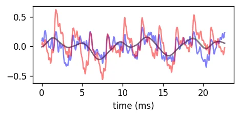
# time-domain excerpt: a short ~23 ms window (1000 samples) from the middle of the clip
td_len = 1000
td_start = n_samples // 2
td_sl = slice(td_start, td_start + td_len)
td_t = np.arange(td_len) / fs * 1e3                        # ms
print('time-domain colors:  ch1 original = blue,  ch1 reconstructed = green,  '
      'ch2 original = red,  ch2 reconstructed = purple')

print('original (channel 0)')
display(make_spectrogram(x[0]))
rd_clip = []
for n_ch in ops:
    partial = models[n_ch]
    with torch.no_grad():
        lq = [z.round().clamp(-127, 127).to(torch.int8) for z in partial.encode(x_in)]
    blob_g = encode_latents(lq)
    ld = decode_latents(blob_g, partial.scale_groups)
    with torch.no_grad():
        xh = partial.decode([z.to(device) for z in ld]).clamp(-1, 1)[0].float().cpu()
    kbps_g = len(blob_g) * 8 / (n_samples / fs) / 1000
    cr_g = 16 * config.input_channels * n_samples / (len(blob_g) * 8)
    psnr_g = -10 * torch.nn.functional.mse_loss(x / 2 + 0.5, xh / 2 + 0.5).log10().item()
    rd_clip.append((kbps_g, psnr_g, n_ch, xh))
    print(f'{n_ch:>2} ch:  {kbps_g:8.2f} kbps   CR={cr_g:8.1f}x   PSNR={psnr_g:.2f} dB')
    plt.figure(figsize=(4, 2), dpi=120)
    plt.plot(td_t, x[0, td_sl].numpy(), alpha=0.5, c='b')
    plt.plot(td_t, xh[0, td_sl].numpy(), alpha=0.5, c='g')
    plt.plot(td_t, x[1, td_sl].numpy(), alpha=0.5, c='r')
    plt.plot(td_t, xh[1, td_sl].numpy(), alpha=0.5, c='purple')
    plt.xlabel('time (ms)'); plt.tight_layout(); plt.show()
    display(make_spectrogram(xh[0]))
    display(Audio(xh.numpy(), rate=fs))

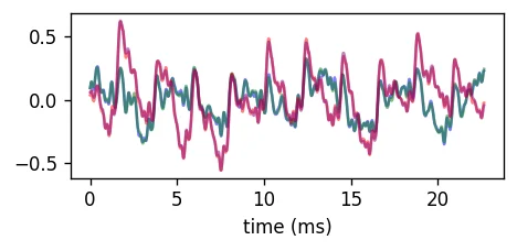
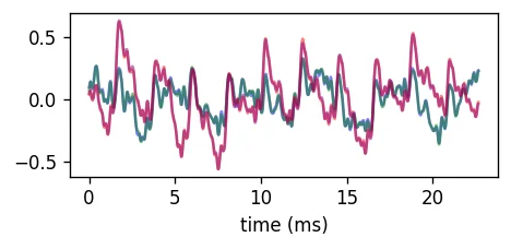
time-domain colors:  ch1 original = blue,  ch1 reconstructed = green,  ch2 original = red,  ch2 reconstructed = purple
original (channel 0)

 4 ch:      2.11 kbps   CR=   669.4x   PSNR=22.53 dB

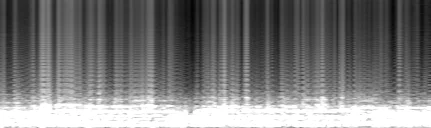
 9 ch:      4.47 kbps   CR=   315.8x   PSNR=25.33 dB

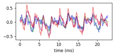
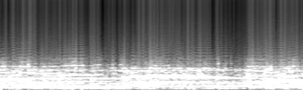
15 ch:      9.57 kbps   CR=   147.4x   PSNR=28.73 dB

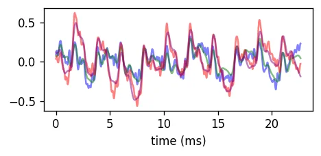
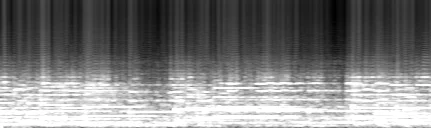
21 ch:     24.54 kbps   CR=    57.5x   PSNR=32.42 dB

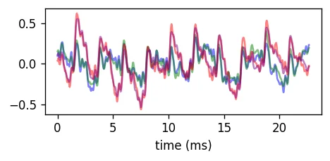
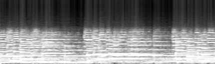
33 ch:     81.08 kbps   CR=    17.4x   PSNR=42.20 dB

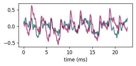
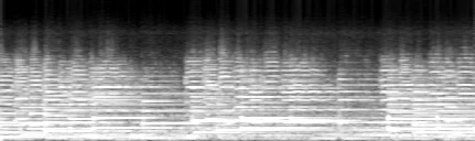
42 ch:    130.39 kbps   CR=    10.8x   PSNR=43.38 dB

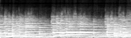
51 ch:    239.62 kbps   CR=     5.9x   PSNR=45.68 dB

Rate–distortion (this clip vs full musdb validation set)

The single clip above shows the workflow; the operating curve below is the full-validation average over all 262 musdb_segments clips, read from results/frappe_v2_audio/rate_distortion_*.json (produced by python -m compressors.frappe_v2_audio.evaluate_rate_distortion). The rate is taken from the mean compression ratio and converted to kbps via kbps = 16·2·fs / CR / 1000 (int16 stereo PCM is 1411.2 kbps). The demo clip is a single excerpt, so its curve sits off the average — the 262-clip mean is the codec’s reported operating point.

import json, glob
rd_path = sorted(glob.glob('results/frappe_v2_audio/rate_distortion_*.json'))[-1]
rd = json.load(open(rd_path))
qs = rd['quality_values']
val_cr   = [rd['results'][str(q)]['mean']['CR'] for q in qs]
val_psnr = [rd['results'][str(q)]['mean']['PSNR_dB'] for q in qs]
pcm_kbps = 16 * config.input_channels * fs / 1000          # 1411.2 kbps for int16 stereo
val_kbps = [pcm_kbps / cr for cr in val_cr]                 # kbps from the mean compression ratio

plt.figure(figsize=(6.5, 4), dpi=120)
plt.semilogx(val_kbps, val_psnr, 'o-', label=f"full validation set ({rd['n_samples']} clips)")
plt.semilogx([p[0] for p in rd_clip], [p[1] for p in rd_clip], 's--', alpha=0.6,
             label=f'demo clip (#{CLIP_INDEX})')
for q, kbv, psv in zip(qs, val_kbps, val_psnr):
    plt.annotate(f'{q}ch', (kbv, psv), fontsize=7, xytext=(3, -8), textcoords='offset points')
plt.xlabel('kbps'); plt.ylabel('PSNR (dB)')
plt.title('FRAPPE v2 audio — PSNR vs kbps (musdb)')
plt.grid(True, alpha=0.3); plt.legend(fontsize=8); plt.tight_layout(); plt.show()

print(f'Full-validation average (from {rd_path.split("/")[-1]}):')
for q, kb, cr, ps in zip(qs, val_kbps, val_cr, val_psnr):
    print(f'  {q:>2} ch:  {kb:8.2f} kbps   CR={cr:8.1f}x   PSNR={ps:.2f} dB')

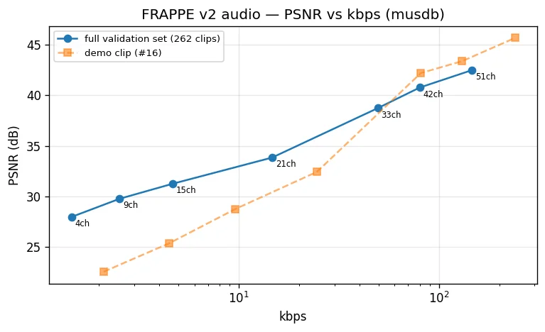
Full-validation average (from rate_distortion_1782557426.json):
   4 ch:      1.46 kbps   CR=   967.3x   PSNR=27.96 dB
   9 ch:      2.54 kbps   CR=   556.1x   PSNR=29.76 dB
  15 ch:      4.65 kbps   CR=   303.2x   PSNR=31.24 dB
  21 ch:     14.66 kbps   CR=    96.2x   PSNR=33.84 dB
  33 ch:     49.38 kbps   CR=    28.6x   PSNR=38.73 dB
  42 ch:     80.08 kbps   CR=    17.6x   PSNR=40.77 dB
  51 ch:    145.66 kbps   CR=     9.7x   PSNR=42.49 dB

Spatial quality (SSDR / SRDR) — FRAPPE vs MP3 / Opus

from torchcodec.encoders import AudioEncoder
from torchcodec.decoders import AudioDecoder
from compressors.audio_eval import align_length
from compressors.spatial_audio_quality import ssdr_srdr

def frappe_psnr(ref, est):
    return -10 * torch.nn.functional.mse_loss(ref / 2 + 0.5, est / 2 + 0.5).log10().item()

def spatial_row(name, kbps_pt, est):
    est = est.float().cpu()
    m = ssdr_srdr(x, est, fs)                       # SSDR/SRDR are scale-invariant ratios
    return (name, kbps_pt, frappe_psnr(x, est), m['SSDR'], m['SRDR'])

# Reference codecs: MP3 + Opus at the target bitrate below on the SAME clip (actual bitrate runs
# higher than the target, which is fine). torchcodec's AudioEncoder expects float samples already
# in [-1, 1] -- exactly how x is peak-normalized (peak just under 1.0, so no clipping) -- so we
# feed x directly with no rescaling, matching the full-scale signal FRAPPE is evaluated on.
target_bit_rate = 1000
enc = AudioEncoder(x, sample_rate=fs)
op_blob = enc.to_tensor(format='opus', bit_rate=target_bit_rate, sample_rate=48_000)
mp_blob = enc.to_tensor(format='mp3',  bit_rate=target_bit_rate)
x_opus = align_length(AudioDecoder(op_blob.numpy().tobytes(), sample_rate=fs).get_all_samples().data, n_samples)
x_mp3  = align_length(AudioDecoder(mp_blob.numpy().tobytes(), sample_rate=fs).get_all_samples().data, n_samples)
op_kbps = 8 * len(op_blob) / 1000 / (n_samples / fs)
mp_kbps = 8 * len(mp_blob) / 1000 / (n_samples / fs)

rows  = [spatial_row('Opus', op_kbps, x_opus), spatial_row('MP3', mp_kbps, x_mp3)]
rows += [spatial_row(f'FRAPPE {nch}ch', kb, xh) for (kb, ps, nch, xh) in rd_clip]   # every truncation rate

print(f'{"codec":>13} {"kbps":>8} {"PSNR":>7} {"SSDR":>7} {"SRDR":>7}')
print('-' * 46)
for name, kb, p, ssdr, srdr in rows:
    print(f'{name:>13} {kb:8.1f} {p:7.2f} {ssdr:7.2f} {srdr:7.2f}')

# Audio + time-domain + TF visualizations for the reference codecs.
print('\ntime-domain colors:  ch1 original = blue,  ch1 reconstructed = green,  '
      'ch2 original = red,  ch2 reconstructed = purple')
for name, kbps_pt, est in [('Opus', op_kbps, x_opus), ('MP3', mp_kbps, x_mp3)]:
    est = est.float().cpu()
    print(f'{name} ({kbps_pt:.1f} kbps)')
    plt.figure(figsize=(4, 2), dpi=120)
    plt.plot(td_t, x[0, td_sl].numpy(), alpha=0.5, c='b')
    plt.plot(td_t, est[0, td_sl].numpy(), alpha=0.5, c='g')
    plt.plot(td_t, x[1, td_sl].numpy(), alpha=0.5, c='r')
    plt.plot(td_t, est[1, td_sl].numpy(), alpha=0.5, c='purple')
    plt.title(f'{name} ({kbps_pt:.1f} kbps) — time domain', fontsize=9)
    plt.xlabel('time (ms)'); plt.tight_layout(); plt.show()
    display(make_spectrogram(est[0]))
    display(Audio(est.numpy(), rate=fs))

        codec     kbps    PSNR    SSDR    SRDR
----------------------------------------------
         Opus      5.7   18.34    1.76  -10.91
          MP3     32.7   33.84   21.18   13.06
   FRAPPE 4ch      2.1   22.53    2.48   -1.35
   FRAPPE 9ch      4.5   25.33    7.21    4.06
  FRAPPE 15ch      9.6   28.73   14.81    7.34
  FRAPPE 21ch     24.5   32.42   19.19   11.91
  FRAPPE 33ch     81.1   42.20   42.08   21.25
  FRAPPE 42ch    130.4   43.38   43.47   22.42
  FRAPPE 51ch    239.6   45.68   49.02   24.73

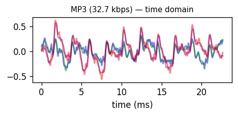
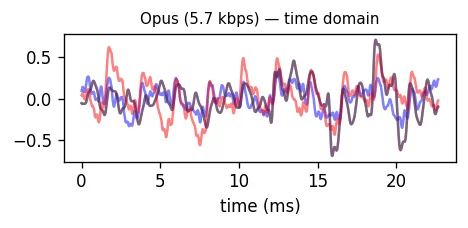
time-domain colors:  ch1 original = blue,  ch1 reconstructed = green,  ch2 original = red,  ch2 reconstructed = purple
Opus (5.7 kbps)

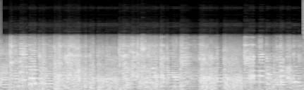
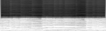
MP3 (32.7 kbps)